Autoregressive (AR) processes are a popular choice for modeling time-varying processes. AR processes are typically written down as a set of conditional distributions, but if we do some algebra we can show how they can also be written as a Gaussian process. One reason having a Guassian process representation is useful is because it makes it more clear how an AR process can be incorporated into larger models, like a spatio-temporal model. In this post, we’ll start with defining an AR process and deriving its mean and variance, then we’ll derive its joint distribution, which is a Gaussian process.
AR processes
Let \(\mathbf{Y} = \left\{ Y_1, Y_2, \dots, Y_n \right\}\) be a set of random variables indexed by time. An aurogressive model assumes that \(\mathbf{Y}\) is correlated over time. An AR model is typically described by defining \(Y_t\) in terms of \(Y_{t-1}\):
\[ Y_{t} = \rho Y_{t-1} + \epsilon_{t} \] where \(\epsilon_{t}\sim N\left(0,\sigma_{\epsilon}^{2}\right)\) and \(\rho \in \mathbb{R}\) is a parameter that controls the degree to which \(Y_t\) is correlated with \(Y_{t-1}\). This model is called an AR process of order 1 because \(Y_t\) only depends on \(Y_{t-1}\).
We can also rearrange terms to emphasize that this representation defines the conditional distribution of \(Y_{t}\) given \(Y_{t-1}\):
\[ \begin{aligned} Y_{t} \vert Y_{t-1} \sim& N(\rho Y_{t-1}, \sigma_\epsilon^2) \\ Y_1 \sim& N(0, \frac{\sigma_\epsilon^2}{1-\rho^2}) \end{aligned} \]
Where the variance of \(Y_1\) comes from the unconditional variance, which is derived below. The stationarity condition of an AR process is that each \(Y_t\) has the same distribution; that is, \(\mu = \mathrm{E}(Y_i) = \mathrm{E}Y_j\) and \(\sigma^2 = \mathrm{Var}(Y_i) = \mathrm{Var}(Y_j)\) for all \(i, j\).
Now we can derive the unconditional mean and variance of \(Y_t\):
\[ \begin{aligned} \mathrm{E}\left(Y_{t}\right) &= \mathrm{E}\left(\rho Y_{t - 1} + \epsilon_{t} \right)\\ &= \rho \mathrm{E}\left( Y_{t - 1 } \right)\\ \mu &= \rho\mu\ \text{(apply stationarity condition)} \\ \mu &= 0 \\ \mathrm{Var}\left(Y_{t}\right) &= \mathrm{Var}\left(\rho Y_{t-1} + \epsilon_{t}\right)\\ &= \rho^{2}\mathrm{Var}(Y_{t-1}) + \mathrm{Var}\left(\epsilon_{t}\right)\\ &= \rho^{2}\mathrm{Var}(Y_{t-1}) + \sigma_{\epsilon}^{2}\\ \sigma^{2} &= \rho^{2}\sigma^{2} + \sigma_{\epsilon}^{2}\ \text{(apply stationarity condition)}\\ \sigma^{2}\left(1-\rho^{2}\right) &= \sigma_{\epsilon}^{2}\\ \sigma^{2} &= \frac{\sigma_{\epsilon}^{2}}{1 - \rho^{2}} \end{aligned} \]
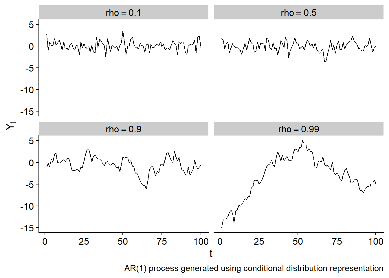
The plot below shows several examples of draws from an AR(1) process with differing values of \(\rho\) and \(\sigma^2_\epsilon = 1\):
Gaussian processes
Gaussian processes model a set of variables as being multivariate normally distributed with mean \(\boldsymbol{\mu}\) and variance/covariance matrix \(\boldsymbol{\Sigma}\):
\[ \mathbf{Y} \sim MVN(\boldsymbol{\mu}, \boldsymbol{\Sigma}) \]
Usually the mean vector is set to \(\boldsymbol{0}\), which means the Gaussian process is fully defined by its choice of variance/covariance matrix \(\boldsymbol{\Sigma}\). The variance/covariance matrix is defined by a kernel function which defines the covariance between any two variables:
\[ \Sigma_{i,j} = K(i, j) \]
An AR(1) process is a Gaussian process
We want to show that an AR process can be represented as a Gaussian process. To do this, we need to show that \(\mathbf{Y}\) is jointly normally distributed with some mean vector and variance/covariance matrix.
We already know that \(\mathrm{E}(Y_t)=0\), so the mean vector of its joint distribution will be \(\mathbf{0}\).
To find the variance/covariance matrix, we need to derive the covariance between \(Y_{t_1}\) and \(Y_{t_2}\). First, let’s consider the simpler case of the covariance between \(Y_t\) and \(Y_{t+1}\):
\[ \begin{aligned} \mathrm{cov}(Y_{t}, Y_{t+1}) &= \mathrm{E} \left[ \left( Y_t - \mathrm{E}[Y_t] \right) \left( Y_{t+1} - \mathrm{E}[Y_{t+1}] \right) \right] \text{ (definition of covariance) } \\ &= \mathrm{E} \left[ Y_t Y_{t+1} \right] \text{ (because } \mathrm{E}[Y_t] = \mathrm{E}[Y_{t+1}] = 0 \text{)} \\ &= \mathrm{E} \left[ Y_t \left( \rho Y_{t} + \epsilon_{t+1} \right) \right] \\ &= \mathrm{E} \left[ \rho Y_t^2 + Y_t \epsilon_{t+1} \right] \\ &= \rho \mathrm{E}\left[ Y_t^2 \right] \\ &= \rho (\mathrm{Var}(Y_t) + \mathrm{E}[Y_t]^2) \\ &= \rho \frac{\sigma_\epsilon^2}{1 - \rho^2} \end{aligned} \]
for \(Y\)s separated by more than one time point, iterating the above result yields the expression
\[ \begin{aligned} \mathrm{cov}(Y_{t_1}, Y_{t_2}) = \rho^{\vert t_1 - t_2 \vert} \frac{\sigma_\epsilon^2}{1 - \rho^2} \end{aligned} \]
Now we can fully define the joint distribution of \(\mathbf{Y}\):
\[ \mathbf{Y} \sim MVN(\mathbf{0}, \boldsymbol{\Sigma}) \]
where \(\Sigma_{i,j} = \rho^{\vert i - j \vert} \frac{\sigma_\epsilon^2}{1-\rho^2}\). This is a Gaussian process!
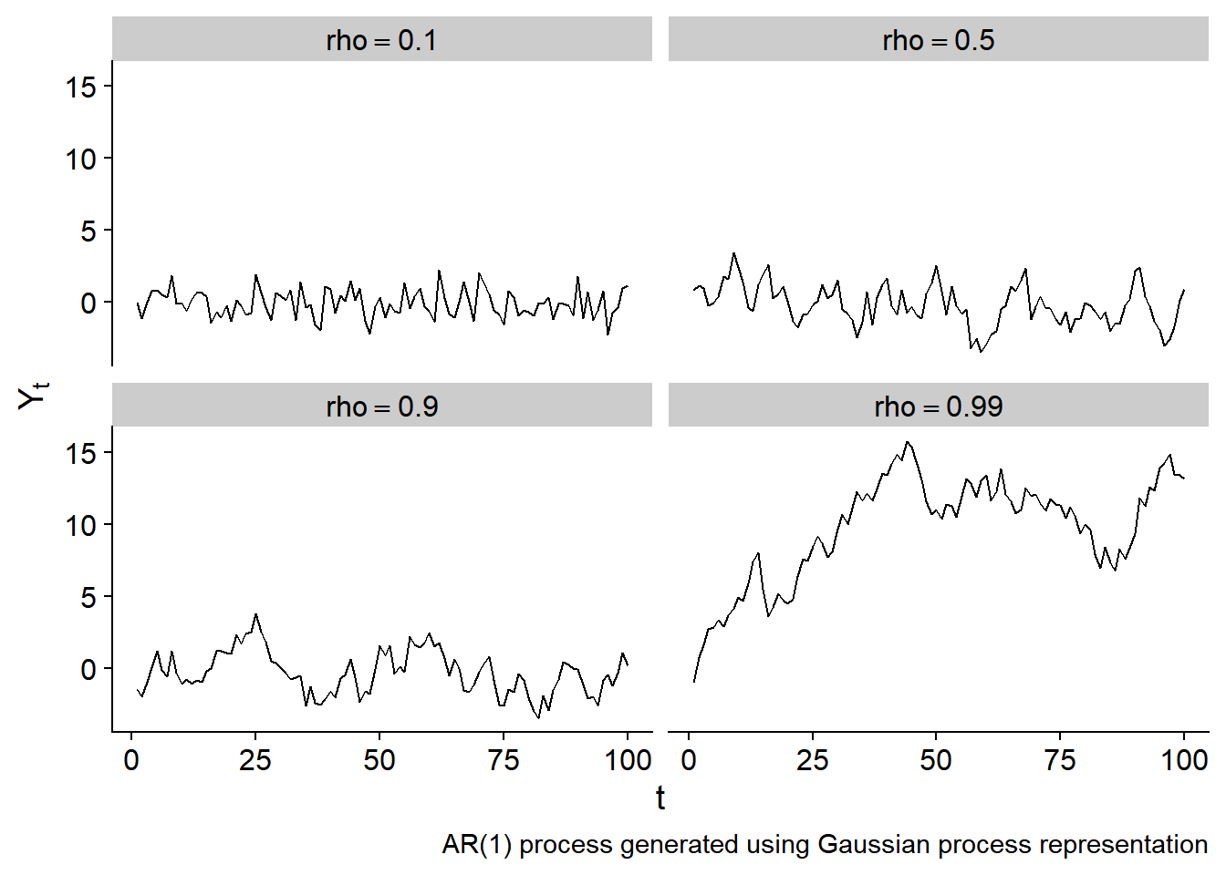
Combining kernel functions
The nice thing about Gaussian processes is that we can combine multiple kernel functions to model processes with dependence from different sources. Two ways kernels can be combined are by multiplication and addition. Multiplying two kernels is like an “AND” operation: the correlation between points will be high if the correlation from both kernels is high. Adding two kernels together is like an “OR” operation: correlation is high if either kernel indicates high covariance.
As an example, let’s build a Gaussian process that combines an AR process (for temporal correlation) and a spatial process (for spatial correlation) by combining two kernel functions. First, we need to define an outcome variable \(Y\) that varies in time and space: let \(Y_{c,t}\) be a random variable indexed by spatial site \(c\) at timepoint \(t\). We take the AR covariance as the first kernel function, to model temporal correlation:
\[ K_1(i, j) = \rho^{\vert t_i - t_j \vert} \frac{\sigma_\epsilon^2}{1 - \rho^2} \]
and a squared-exponential kernel function to model spatial dependence:
\[ K_2(i, j) = \alpha^2 \exp\left( -\frac{d(i, j)}{2\lambda^2} \right) \]
where \(d(i, j)\) is the spatial distance between sites \(i\) and \(j\), \(\lambda\) is a length-scale parameter, and \(\alpha^2\) is a parameter controlling the magnitude of the covariance.
Combine the two kernel functions so that two data points are correlated if they are close together in time and space:
\[ \begin{aligned} K(i, j) &= K_1(i, j) \times K_2(i, j) \\ &= \rho^{\vert t_i - t_j \vert} \frac{\sigma_\epsilon^2}{1 - \rho^2} \alpha^2 \exp\left( -\frac{d(i, j)}{2\lambda^2} \right) \end{aligned} \]
Note the parameters \(\sigma^2_\epsilon\) and \(\alpha^2\), which are multipled together, would be unidentifiable in parameter estimation and should be replaced by a single parameter that controls the magnitude of the covariance.
To illustrate this Gaussian process model, I started by generating a set of sites with random locations:
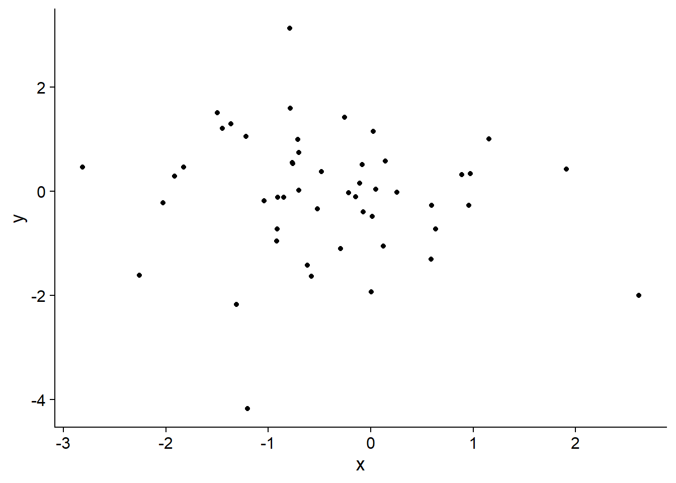
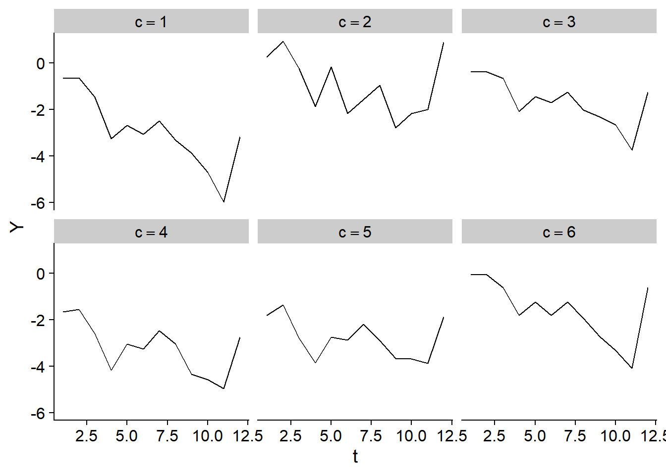
then I drew from the Gaussian process using the parameters temporal parameters \(\rho=0.9\), \(\sigma_\epsilon^2=1\) and spatial parameters \(\alpha = 1\) and \(\lambda=2\).
The plot below shows the time trend in the first six sites:
And the spatial distribution over time of \(Y_{c,t}\) is shown below:
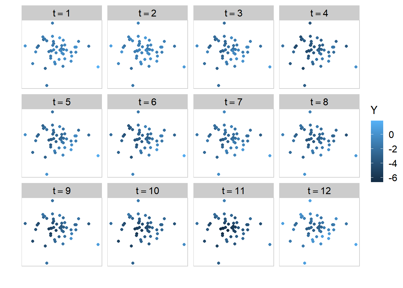
Visually we can see that the Gaussian process generates data that is correlated in both time and space.
Modeling using the mean and the covariance
The spatio-temporal Gaussian process we defined in the previous section does its modeling through the variance/covariance matrix, with its mean function set to zero. An alternative way to think about a spatio-temporal process is akin to the first AR representation we looked at, and define \(\mathbf{Y}_t\) (the set of all \(Y_{c,t}\) at time \(t\)) relative to \(\mathbf{Y}_{t-1}\):
\[ \begin{aligned} \mathbf{Y}_{t} = \rho \mathbf{Y}_{t-1} + \boldsymbol{\epsilon}_t \end{aligned} \]
where \(\boldsymbol{\epsilon_t} \sim MVN(\mathbf{0}, \boldsymbol{\Sigma}_\epsilon)\).
If we set \(\boldsymbol{\Sigma_\epsilon}\) to be the diagonal matrix \(\boldsymbol{\Sigma}_\epsilon = \sigma^2_\epsilon \mathbf{I}_n\) then we will have an independent AR(1) independent process for each spatial site. It gets more interesting if we define \(\boldsymbol{\Sigma}_\epsilon\) by a covariance function so we can include dependence between sites, for example dependence based on the distance between the sites. For now, let’s use the squared exponential kernel and define \(\Sigma_{i,j} = \alpha^2 \exp\left(-\frac{d(i, j)}{2\lambda^2} \right)\).
Is this process also equivalent to a mean zero Gaussian process with some covariance kernel? We’ll answer this question by deriving the covariance between any two points.
The mean of \(\mathbf{Y_t}\) can be shown to be zero in the same way we showed a univariate AR process has mean 0. We also need to know the overall variance/covariance matrix of \(\mathbf{Y}_t\), which we’ll call \(\boldsymbol{\Phi}\); the logic is imilar to the univariate case, and I’ll show it here for completeness:
\[ \begin{aligned} \mathrm{Var}\left(\boldsymbol{Y}_{t}\right) & =\mathrm{Var}\left(\rho^{2}\mathbf{Y}_{t-1} + \boldsymbol{\epsilon}_{t}\right) \\ &= \rho^{2}\mathrm{Var}\left(\boldsymbol{Y}_{t-1}\right)+\mathrm{Var}\left(\boldsymbol{\epsilon}_{t}\right) \\ \boldsymbol{\Phi} & =\rho^{2}\boldsymbol{\Phi}+\boldsymbol{\Sigma}_\epsilon \\ \boldsymbol{\Phi}-\rho^{2}\boldsymbol{\Sigma} &= \boldsymbol{\Sigma}_\epsilon \\ \boldsymbol{\Phi}\left(\mathbf{I}-\rho^{2}\mathbf{I}\right) & =\boldsymbol{\Sigma}_\epsilon \\ \boldsymbol{\Phi} &=\boldsymbol{\Sigma}_{\epsilon}\left(\mathbf{I}-\rho^{2}\mathbf{I}\right)^{-1} \end{aligned} \]
If we pull out two sites at the same time point, their covariance is \(\mathrm{cov}(Y_{t,c_1}, Y_{t,c_2}) = \frac{\Sigma_{\epsilon, c_1, c_2}}{1-\rho^2}\), which looks very similar to the unidimensional AR(1) process variance.
Now we derive the covariance between any two sites that are one time point apart:
\[ \begin{aligned} \mathrm{cov}\left(y_{c_1,t},y_{c_2,t+1}\right) & =\mathrm{E}\left[\left(y_{c_1,t}-\mathrm{E}\left[y_{c_1,t}\right]\right)\left(y_{c_2,t}-\mathrm{E}\left[y_{c_2,t}\right]\right)\right]\\ & =\mathrm{E}\left[y_{c_1,t}y_{c_2,t}\right]\\ & =\mathrm{E}\left[y_{c_1,t}\left[\rho y_{c_2,t}+\epsilon_{c_2,t+1}\right]\right]\\ & =\rho\mathrm{E}\left[y_{c_1,t}y_{c_2,t}\right]\\ & =\rho\mathrm{cov}\left(y_{c_1,t}y_{c_2,t}\right)\\ & =\rho\frac{\Sigma_{i,j}}{1-\rho^2} \\ &= \rho \frac{1}{1-\rho^2} \Sigma_{i,j} \\ &= \rho \frac{1}{1-\rho^2} \alpha^2 \exp\left(-\frac{d(i, j)}{2\lambda^2} \right) \end{aligned} \]
for sites more than one time point away from each other, we can iterate the above result to get a general expression of the covariance between any two points:
\[ \begin{aligned} \mathrm{cov}\left(y_{c_1,t_1},y_{c_2,t_2}\right) &= \rho^{\vert t_1 - t_2 \vert}\frac{1}{1-\rho^2} \alpha^2 \exp\left(-\frac{d(i, j)}{2\lambda^2} \right) \end{aligned} \]
if we reparameterize \(\alpha\) to be the product of two parameters \(\alpha = \sigma^2_\epsilon \alpha\), we get
\[ \begin{aligned} \mathrm{cov}\left(y_{c_1,t_1},y_{c_2,t_2}\right) &= \rho^{\vert t_1 - t_2 \vert}\frac{\sigma^2_\epsilon}{1-\rho^2} \alpha^2 \exp\left(-\frac{d(i, j)}{2\lambda^2} \right) \\ &= K_1(i, j) \times K_2(i,j) \end{aligned} \]
which is the product of an AR(1) and squared exponential kernel function as defined in the previous section. In practice we wouldn’t want to separate these parameters because both of them will not be identifiable given observed data, but I separated them here to show how the covariance structure is the product of two kernel functions.
Therefore, we can write this process in the form of a Gaussian process with mean zero and covariance kernel given by the product of a temporal and spatial kernel:
\[ \begin{aligned} \mathbf{Y} \sim& MVN(\mathbf{0}, \boldsymbol{\Sigma}) \\ \Sigma_{i,j} =& K_1(i, j) \times K_2(i, j) \end{aligned} \]
The spatio-temporal processes defined as a set of conditional distributions and as a Gaussian process are equivalent.
To summarize, AR processes can be written as a Gaussian process model, which is useful because a temporal process can then be easily combined with other sources of dependence. In general, we can build our models by defining conditional distributions with a given mean and covariance, or a joint distribution with mean zero where the model is fully defined by a variance/covariance kernel function. In a future post I will look at Bayesian parameter estimation in these models using Stan.