Presidential Primary Polling Analysis in Stan

Note: this post has been updated with more recent data.

I often use random walk/autoregressive models in my research as a component in time-series analysis, and I wanted to get some more experience fitting them to data. FiveThirtyEight publishes several polling datasets, including polling for the 2020 Democratic presidential primary. I used Stan to fit a Bayesian random walk model to the polling data, which I describe below. The Stan and R code used in this post is available as a Github gist.

Let \(\delta_{c,t}\) be the true proportion of voters in favor of candidate \(c\) at time \(t\). Our modeling assumption is that the logit-transform of \(\delta_{c,t}\) follows a random walk; that is: \[ \mathrm{logit}(\delta_{c,t}) \sim \mathrm{N}\left(\mathrm{logit}(\delta_{c,t-1}), \tau^2\right) \] We can’t observe \(\delta_{c,t}\) directly; we have to infer it through the noisy observations we have from polls.

Let \(s_{i}\) be the sample size of poll \(c[i]\) and \(y_{i}\) the number of poll respondents in favor of candidate \(c[i]\) at time \(t[i]\). Let \(\phi_i\) be the proportion of poll respondents in favor of candidate \(c[i]\) at time \(t[i]\). To incorporate sampling error, we model \(y_i\) as binomial: \[ y_i \sim \mathrm{Binomial}(s_i, \phi_i) \] We also allow for added variance in our observations by relating \(\phi_i\) to the true logit proportion \(\delta_{c[i], t[i]}\) with a normal distribution: \[ \mathrm{logit}(\phi_i) \sim \mathrm{N}(\mathrm{logit}(\delta_{c[i], t[i]}), \sigma^2) \]

To finish defining the model half-normal priors on the hyperparameters. The prior for \(\tau^2\) has a small variance to improve identification of the model (a vaguer prior can cause the MCMC chains to not mix well.) \[ \begin{aligned} \tau^2 &\sim \mathrm{N}(0, 0.02)[0, \infty] \\ \sigma^2 &\sim \mathrm{N}(0, 1)[0, \infty] \end{aligned} \]

Here is the Stan representation of the statistical model:

S4 class stanmodel 'random_walk' coded as follows:
data {
  int<lower=0> T; // Number of timepoints
  int<lower=0> C; // Number of candidates
  int<lower=0> N; // Number of poll observations
  
  int sample_size[N]; // Sample size of each poll
  int y[N]; // Number of respondents in poll for candidate (approximate)
  int<lower=1, upper=T> get_t_i[N]; // timepoint for ith observation
  int<lower=1, upper=C> get_c_i[N]; // candidate for ith observation
}
parameters {
  matrix[C, T] delta_logit; // Percent for candidate c at time t
  real<lower=0, upper=1> phi[N]; // Percent of participants in poll for candidate
  real<lower=0> tau; // Random walk variance
  real<lower=0,upper=0.5> sigma; // Overdispersion of observations
}
model {
  // Priors
  tau ~ normal(0, 0.2);
  sigma ~ normal(0, 1);
  
  // Random walk
  for(c in 1:C) {
    delta_logit[c, 2:T] ~ normal(delta_logit[c, 1:(T - 1)], tau);
  }
  
  // Observed data
  y ~ binomial(sample_size, phi);
  for(i in 1:N) {
    // Overdispersion
    delta_logit[get_c_i[i], get_t_i[i]] ~ normal(logit(phi[i]), sigma);
  }
}
generated quantities {
  matrix[C, T] delta = inv_logit(delta_logit);
} 

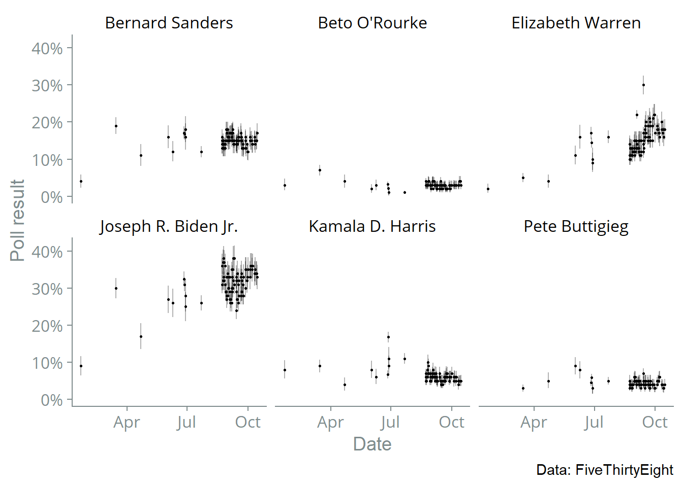
The raw dataset that we are going to fit:

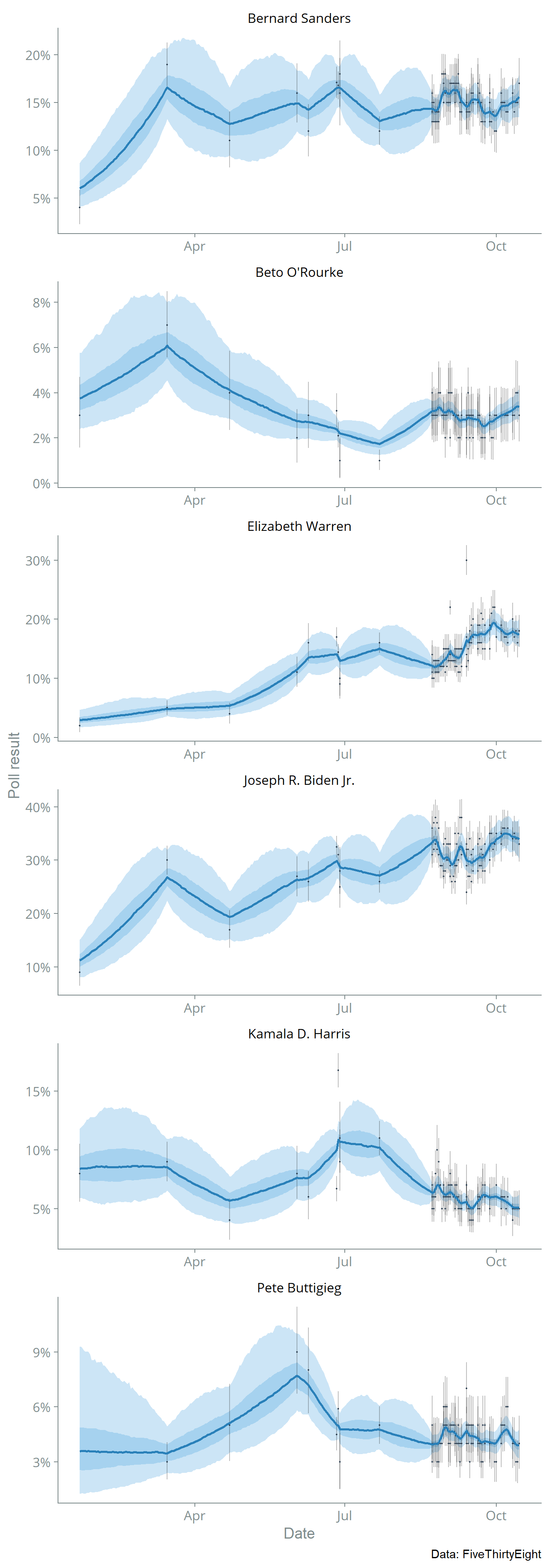
I fitted the Stan model to the data using the standard HMC-NUTS algorithm and 1,000 MCMC iterations (with 500 of those for warmup.) The plot below shows the posterior median with 75% and 95% credible intervals.

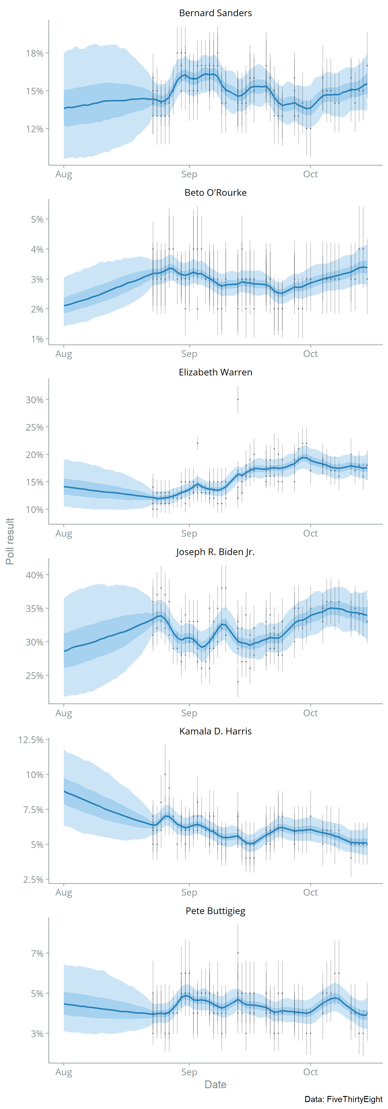
Let’s zoom in on August-November 2019 where there are more data:

This model is too simple to be that useful, but it could serve as a starting point for more complex models. The model could be improved by incorporating more information, perhaps by finding a data source that includes more polls or modifying the model to incorporate results from head-to-head matchups. We might also want to model systematic biases by the type of poll (phone or internet) or the pollster.