
Paul Klee: Joyfal Mountain Landscape (1929)
A Gaussian Process (GP) is a process for which any finite set of observations follows a multivariate normal distribution. GPs are defined by their mean and a kernel function that gives the covariance between any two observations. They are useful in Bayesian statistics as priors over function spaces.
To denote a GP prior over a set of observations \(\bm{y} = \{y_1, y_2, \cdots, y_n\}\) at points \(\bm{x} = \{ x_1, x_2, \cdots, x_n\}\), we write: \[ \bm{y} \sim \mathcal{GP}(\bm{\mu}, \bm{\Sigma}) \]
where the covariance matrix \(\bm{\Sigma}\) is computed via a kernel function \(k(x, x^\prime)\). A popular choice of kernel function that we will consider in this post is the squared exponential kernel: \[ k(x_i, x_j) = \alpha^2 \exp\left(- \frac{(x_i - x_j)^2}{2\ell^2} \right) \]
where \(\alpha\) is a scale parameter and \(\ell\) is a length-scale parameter which controls the strength of the association between points as they become farther apart.
Intuitively, in order to define a GP we need to be able to write down the covariance between any two points.
Let’s write this kernel function in R, and use it to draw samples from a GP. For simplicity, we will fix \(\bm{\mu} = \bm{0}\) for all the GPs we work with in this post. First, define the kernel function:
k <- function(x_i, x_j, alpha, l) {
  alpha^2 * exp(-(x_i - x_j)^2 / (2 * l^2))
}
Let’s write a helper function that, given a kernel and a set of points, generates a full covariance matrix:
covariance_from_kernel <- function(x, kernel, ...) {
  outer(x, x, kernel, ...)
}
and a function to draw from a mean-zero GP with a given covariance kernel:
gp_draw <- function(draws, x, Sigma, ...) {
  mu <- rep(0, length(x))
  mvtnorm::rmvnorm(draws, mu, Sigma)
}
Now we can draw 10 samples from a mean-zero GP with a squared-exponential kernel with parameters \(\alpha=1\), \(l=1\):
n <- 100 # number of points to draw
x <- seq(1, 10, length.out = n) # position of each point

# Kernel parameters
alpha <- 1
l <- 1

set.seed(1)

# Draw 10 samples
Sigma <- covariance_from_kernel(x, k, alpha = alpha, l = l)
y <- gp_draw(10, x, Sigma)

matplot(x, t(y), type = 'l', xlab = 'x', ylab = 'y')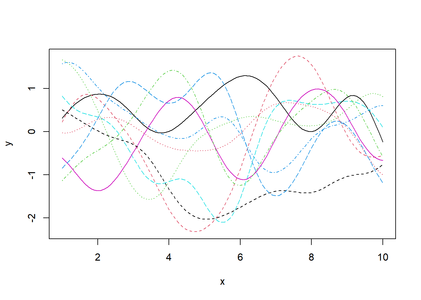
Derivative of a GP
The derivative of a GP is also a GP, with its existence determined by the differentiability of its mean and kernel functions. The squared exponential kernel is infinitely differentiable, so the associated Gaussian Process has infinitely many derivatives.
This derivative is useful because we may have prior knowledge about likely values of the derivative. For example, monotonicity constraints can be encoded as prior knowledge that the derivative is always positive or negative. In other cases we may have direct observations of the derivative that we would like to incorporate into model fitting.
Let \(\bm{y}^\prime = \{ y^\prime_1, y^\prime_2, \cdots, y^\prime_{n^\prime} \}\) be a set of derivative observations. The derivative GP, which we’ll denote \(\mathcal{GP}^\prime\), is given by \[ \bm{y}^\prime \sim \mathcal{GP}^\prime(\frac{d}{dx}\bm{\mu}, \frac{d}{dx}\bm{\Sigma}) \] where the derivative of the covariance matrix is defined by the derivative of the original kernel function with respect to both of its inputs, which we will denote \(k_{11}\) to indicate that both arguments are derivative observations: \[ k_{11}(x_i, x_j) = \frac{\partial}{\partial x_i \ \partial x_j} k(x_i, x_j) = \frac{ \alpha^2 }{ \ell^4 }\left( l^2 - (x_i - x_j)^2 \right) \exp\left( -\frac{(x_i - x_j)^2}{2\ell^2} \right) \]
This is enough information to be able to draw random samples from the derivative of a GP. Let’s write the new kernel \(k_11\) in R, and sample from the derivative GP:
k_11 <- function(x_i, x_j, alpha, l) {
  alpha^2 / l^4 * (l^2 - (x_i - x_j)^2) * exp(-(x_i - x_j)^2 / (2*l^2))
}

n_prime <- 100
x_prime <- seq(1, 10, length.out = n_prime)

# Draw 10 samples
Sigma_prime <- covariance_from_kernel(x_prime, k_11, alpha = alpha, l = l)
y_prime <- gp_draw(10, x_prime, Sigma_prime)

matplot(x_prime, t(y_prime), type = 'l', xlab = 'x', ylab = "y'")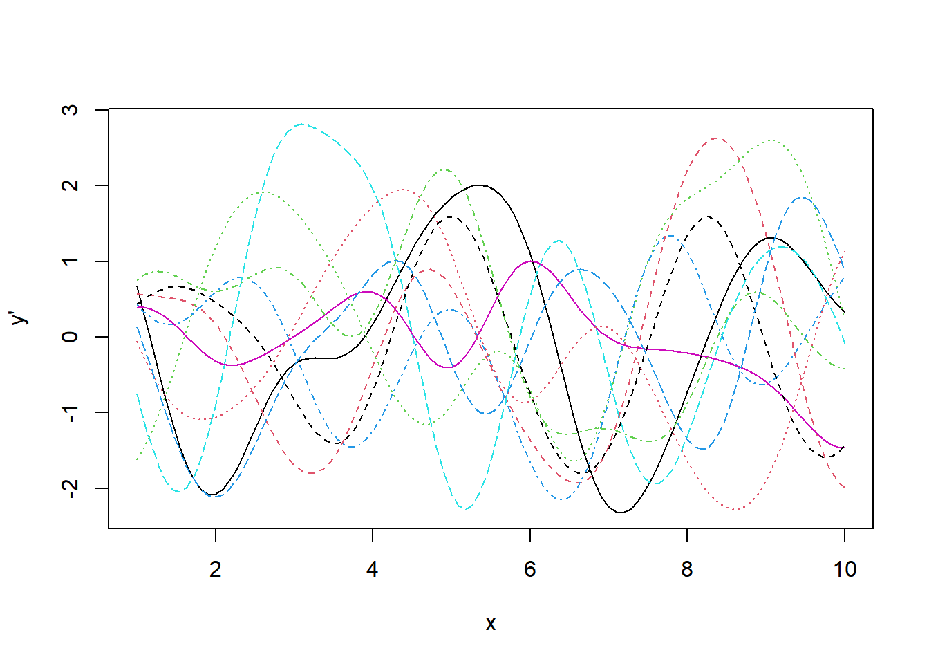
It’s hard to interpret this plot because we can’t compare these derivative values to the corresponding normal GP. Fortunately, it’s possible to sample from the joint distributions of the observations and its derivatives, which is in fact also a GP. To define it, we need to know the covariance between an observation and a derivative observation.
Let \(k_{01}(x_i, x_j)\) be the covariance between an observation at \(x_i\) and a derivative observation at \(x_j\). Then \[ k_{01}(x_i, x_j) = \frac{\alpha^2}{\ell^2} (x_i - x_j) \exp\left( -\frac{(x_i - x_j)^2}{2\ell^2} \right) \]
Similarly, \(k_{10}(x_i, x_j)\) is the covariance between a derivative observation at \(x_i\) and an observation at \(x_j\): \[ k_{10}(x_i, x_j) = \frac{\alpha^2}{\ell^2} (x_j - x_i) \exp\left( -\frac{(x_i - x_j)^2}{2\ell^2} \right) \] As we would expect from the symmetry of covariance matrices, \(k_{01}(x_i, x_j) = k_{10}(x_j, x_i)\). That means we can get away with just defining one of them in R:
k_01 <- function(x_i, x_j, alpha, l) {
  alpha^2 / l^2 * (x_i - x_j) * exp(-(x_i - x_j)^2 / (2*l^2))
}
Now construct a combined vector by concatenating the observations \(y\) and derivative observations \(y^\prime\), denoted \(y^\mathrm{all}\), of length \(n + n^\prime\). Let \(\bm{x}^{\mathrm{all}}\) be the corresponding positions of each observation in \(\bm{y}^{\mathrm{all}}\). Let \(\bm{d}^{\mathrm{all}}\) be a \(n+n^\prime\) length vector where \(d^\mathrm{all}_i = 1\) if \(y^{\mathrm{all}}_i\) is a derivative observation, and \(d^{\mathrm{all}}_i = 0\) if \(y^{\mathrm{all}}_i\) is a normal observation. Then define a new kernel over the joint observations: \[ k^{\mathrm{all}}(x_i, x_j, d_i, d_j) = \begin{cases} k(x_i, x_j) & d_i = 0, d_j = 0 \text{ (both normal observations)} \\ k_{01}(x_i, x_j) & d_i = 0, d_j = 0 \text{ (one derivative, one normal)} \\ k_{10}(x_i, x_j) & d_i = 1, d_j = 0 \text{ (one derivative, one normal)} \\ k_{11}(x_i, x_j) & d_i = 1, d_j = 0 \text{ (both derivatives)} \end{cases} \]
In R:
k_all <- function(x_i, x_j, d_i, d_j, ...) {
  dplyr::case_when(
    d_i == 0 & d_j == 0 ~ k(x_i, x_j, ...),
    d_i == 0 & d_j == 1 ~ k_01(x_i, x_j, ...),
    d_i == 1 & d_j == 0 ~ k_01(x_j, x_i, ...),
    d_i == 1 & d_j == 1 ~ k_11(x_i, x_j, ...),
  )
}
We also need a new function to form the joint covariance matrix:
joint_covariance_from_kernel <- function(x, d, kernel, ...) {
  outer(1:length(x), 1:length(x),
        function(i, j) kernel(x[i], x[j], d[i], d[j], ...))
}
Finally, I’m going to split out the plotting code into a separate function as it gets more complicated than before:
plot_joint_gp <- function(x, y, d) {
  plot(x[d == 0], y[d == 0], type = 'l', ylim = range(y),
       col = 'black', xlab = 'x', ylab = 'y')
  lines(x[d == 1], y[d == 1], type = 'l', col = 'blue', lty = 2)
  abline(h = 0, lty = 3, col = "gray")
  legend('topright', legend = c("GP", "Derivative of GP"),
         col = c("black", "blue"), lty = 1:2)
}
Now we can sample from the joint distribution of the observations and derivatives:
x_all <- c(x, x_prime)
d_all <- c(rep(0, length(x)), rep(1, length(x_prime)))

Sigma_all <- joint_covariance_from_kernel(x_all, d_all, k_all, alpha = alpha, l = l)
y_all <- gp_draw(1, x_all, Sigma_all)

plot_joint_gp(x_all, y_all[1,], d_all)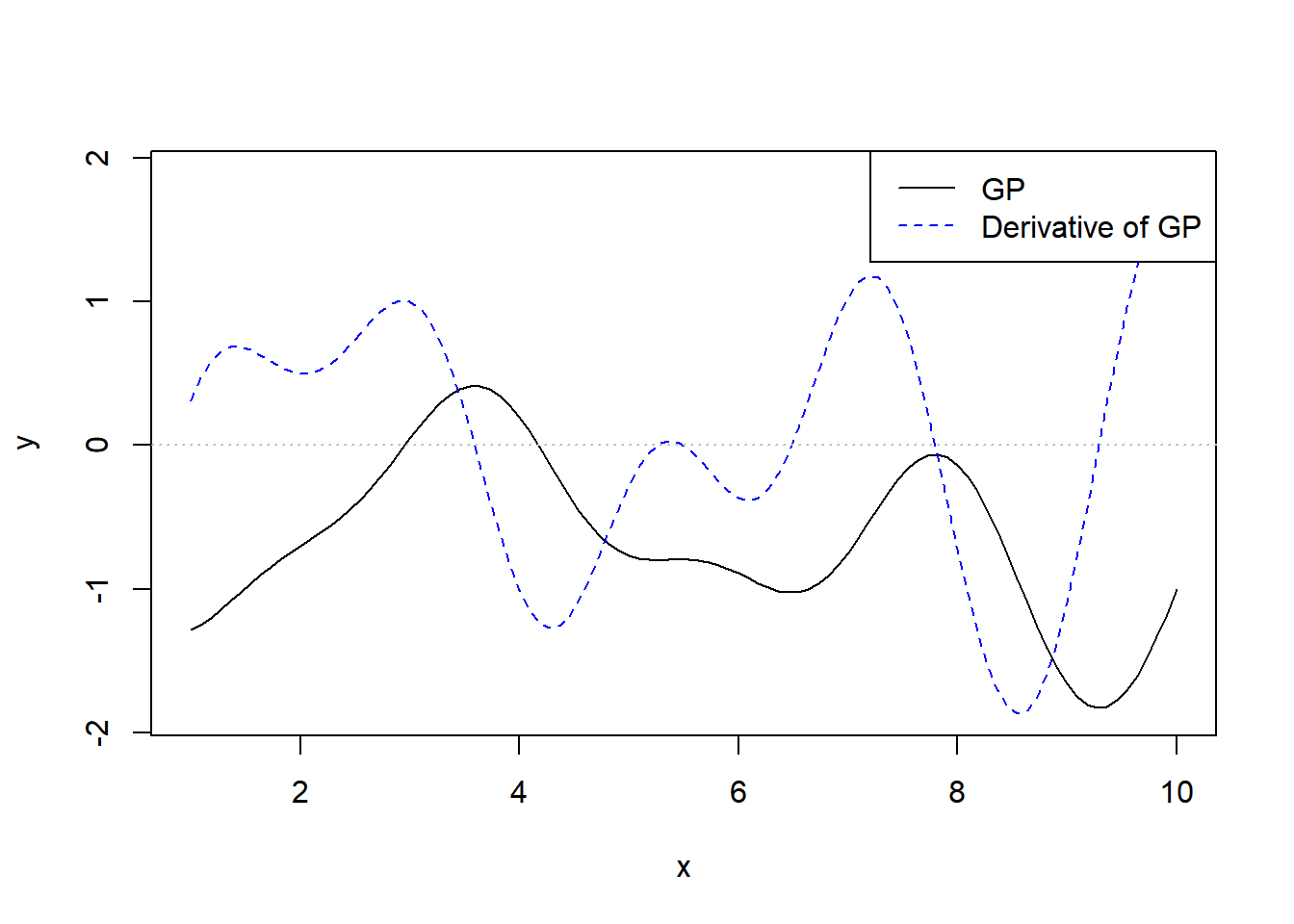
Let’s plot one more:
y_all <- gp_draw(1, x_all, Sigma_all)
plot_joint_gp(x_all, y_all[1,], d_all)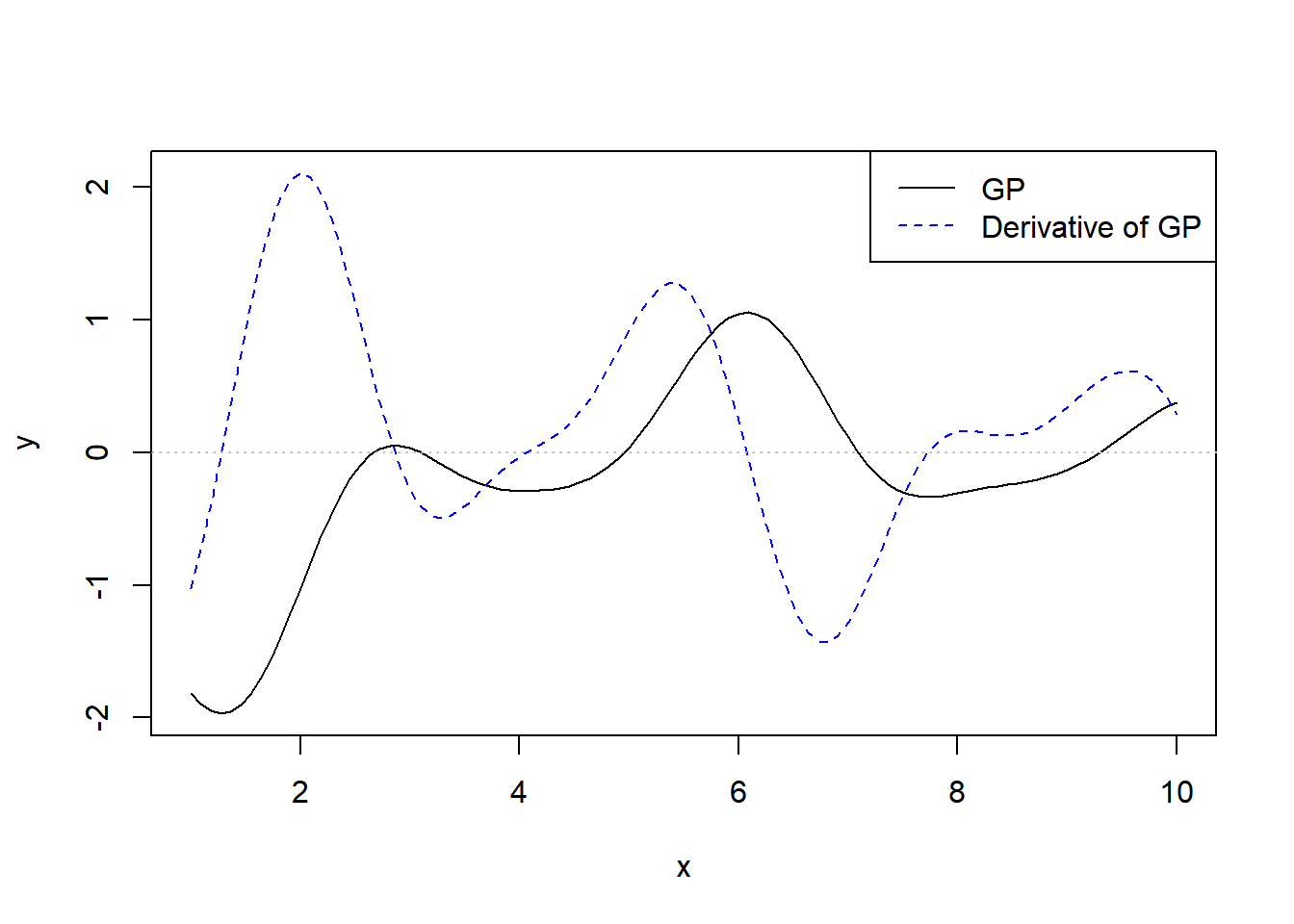
So far we’ve seen how derivatives of GPs are defined, and how to draw from the joint distribution of a GP and its derivative. In future posts we’ll look at fitting GPs in Stan with derivative observations, and at shape-constrained GPs.
References
- Andrew McHutchon, Differentiating Gaussian Processes
- Rasmussen et al. 2006, Gaussian Processes for Machine Learning, Chapter 9