A few years ago, The New York Times published an article about several Major League Baseball players who use the sitcom Friends to improve their English. Friends seems to be a very popular tool for learning English: there’s even an ESL program developed around it, and you can easily find advice on how to use Friends as a language learning tool.
In my own language learning I’ve relied heavily on frequency dictionaries, which order words by their popularity. Learning just the top 500-1,000 words in language goes surprisingly far in conversation.
I wanted to know how many English words someone would need to recognize to be able to watch Friends and understand, say, 90% of all the words.
Here the definition of “word” becomes important. For the purposes of this article, I’m going to consider most grammatical inflections of a root to be the same word. For example, “go”, “going”, and “went” will be considered one word, since they all relate back to the root word “to go”. Later on we’ll see how to operationalize this via lemmatization algorithms, which will allow us to map words back to their grammatical roots.
Fortunately, complete transcripts of Friends are available online. Below I go through the data collection and analysis. But first, here’s the final result:
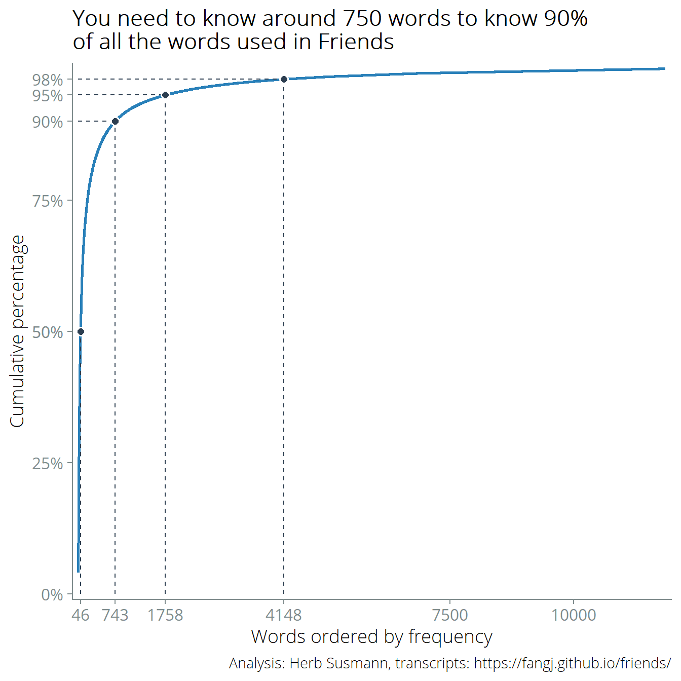
Around 750 words gets you to 90% coverage. Watching Friends where you don’t know every tenth word could be a frustrating experience, but hopefully context clues would help fill in gaps. The Appendix at the bottom of the post lists the top 750 words.
The numbers in this post should be considered as rough estimates because I did not filter out other words that we may not want to consider as words, like proper nouns (“Joey”, “Monica”, “New York”, etc.)
Data Collection
The script of every episode of Friends is available at https://fangj.github.io/friends/. I used rvest to download every file, and parsed the scripts into individual lines. I only wanted to have to do this once, so I saved the results to a CSV file so that subsequent analyses wouldn’t have to redownload all of the data.
library(tidyverse)
library(rvest)

pages <- read_html("https://fangj.github.io/friends/") %>%
  html_nodes("a") %>%
  html_attr("href")

pages <- str_c("https://fangj.github.io/friends/", pages)

parse_episode <- function(url) {
  read_html(url) %>%
    html_nodes("p:not([align=center])") %>%
    .[-1] %>%
    html_text() %>%
    enframe(name = NULL, value = "line") %>%
    mutate(
      url = url,
      episode = str_extract(url, "\\d{4}"), # extract episode number
      character = str_extract(line, "^(\\w+):"), # extract character name
      character = str_replace_all(character, ":$", ""),
      line = str_replace_all(line, "^\\w+: ", ""),
    ) %>%
    filter(line != "")
}

friends_raw <- pages %>% map(parse_episode) %>%
  bind_rows()

write_csv(friends_raw, "./friends.csv")
This yields a raw dataset with the lines from every episode:
head(friends_raw, n = 10) %>%
  select(episode, character, line) %>%
gt::gt()| episode | character | line |
|---|---|---|
| 0101 | NA | [Scene: Central Perk, Chandler, Joey, Phoebe, and Monica are there.] |
| 0101 | Monica | There's nothing to tell! He's just some guy I work with! |
| 0101 | Joey | C'mon, you're going out with the guy! There's gotta be something wrong with him! |
| 0101 | Chandler | All right Joey, be nice. So does he have a hump? A hump and a hairpiece? |
| 0101 | Phoebe | Wait, does he eat chalk? |
| 0101 | NA | (They all stare, bemused.) |
| 0101 | Phoebe | Just, 'cause, I don't want her to go through what I went through with Carl- oh! |
| 0101 | Monica | Okay, everybody relax. This is not even a date. It's just two people going out to dinner and- not having sex. |
| 0101 | Chandler | Sounds like a date to me. |
| 0101 | NA | [Time Lapse] |
Cleaning
First, there are some lines that give stage directions which we want to filter out of the dataset, since we are only interested in spoken words. There are also directions given sometimes within a character’s line, which we want to filter.
friends <- friends_raw %>%
  mutate(
    line = str_replace_all(line, "[\u0091\u0092]", "'"),
    line = str_replace_all(line, "\u0097", "-"),
    line = str_replace_all(line, "\\([\\w\n [[:punct:]]]+\\)", ""),
    line = str_replace_all(line, "\\[[\\w\n [[:punct:]]]+\\]", ""),
    line = str_trim(line)
  ) %>%
  filter(line != "")

head(friends, n = 10) %>%
  select(episode, character, line) %>%
gt::gt()| episode | character | line |
|---|---|---|
| 0101 | Monica | There's nothing to tell! He's just some guy I work with! |
| 0101 | Joey | C'mon, you're going out with the guy! There's gotta be something wrong with him! |
| 0101 | Chandler | All right Joey, be nice. So does he have a hump? A hump and a hairpiece? |
| 0101 | Phoebe | Wait, does he eat chalk? |
| 0101 | Phoebe | Just, 'cause, I don't want her to go through what I went through with Carl- oh! |
| 0101 | Monica | Okay, everybody relax. This is not even a date. It's just two people going out to dinner and- not having sex. |
| 0101 | Chandler | Sounds like a date to me. |
| 0101 | Chandler | Alright, so I'm back in high school, I'm standing in the middle of the cafeteria, and I realize I am totally naked. |
| 0101 | All | Oh, yeah. Had that dream. |
| 0101 | Chandler | Then I look down, and I realize there's a phone... there. |
Now we transform our data from a set of lines from every script into a format that is more useful for analysis. Using tidytext, we generate a new table that has every word from the corpus and how many times it was used. We also calculate cumulative sums and proportions.
# Counts how many times each word
# appears, sorts by number of appearances,
# and adds cumulative proportions
add_cumulative_stats <- function(x) {
  x %>%
    count(word, sort = TRUE) %>%
    mutate(cumsum = cumsum(n),
           cumprop = cumsum / sum(n),
           index = 1:n())
}

library(tidytext)

words <- friends %>%
  unnest_tokens(word, line)

word_counts <- add_cumulative_stats(words)

word_counts %>%
  head(n = 10) %>%
gt::gt()| word | n | cumsum | cumprop | index |
|---|---|---|---|---|
| i | 23298 | 23298 | 0.04076248 | 1 |
| you | 22017 | 45315 | 0.07928371 | 2 |
| the | 13292 | 58607 | 0.10253956 | 3 |
| to | 11554 | 70161 | 0.12275459 | 4 |
| a | 10749 | 80910 | 0.14156118 | 5 |
| and | 9405 | 90315 | 0.15801629 | 6 |
| it | 7631 | 97946 | 0.17136758 | 7 |
| that | 7564 | 105510 | 0.18460166 | 8 |
| oh | 7226 | 112736 | 0.19724436 | 9 |
| what | 6355 | 119091 | 0.20836315 | 10 |
From the cumulative proportions in the table we can see that knowing the top 10 words covers around 20% of all the words in the dataset.
This is a good start, but it’s not quite what we want. Right now the data includes grammatical variations of the same word as different words. For example, “age” and “ages” really represent the same word, but the graph above includes them as two separate words. As such, the data we have so far overestimates the number of unique words that appear in Friends.
Lemmatizing algorithms try to map every grammatical variation of a word to a “stem”. For example, the words “go”, “going”, and “went” should map to the stem “go”. Stemming algorithms are related, but work by removing suffixes from the ends of words. A stemming algorithm wouldn’t know to map “went” to “go”; for that, we need lemmatization, which uses dictionaries to reverse the inflected forms of words to its grammatical root. The package textstem provides a lemmatize_words function in R.
library(textstem)

word_lemmas <- words %>%
  mutate(word = lemmatize_words(word))

word_lemma_counts <- add_cumulative_stats(word_lemmas)
There are 11,852 words after lemmatization, compared to 15,134 before.
word_lemma_counts %>%
  head(n = 10) %>%
gt::gt()| word | n | cumsum | cumprop | index |
|---|---|---|---|---|
| i | 23298 | 23298 | 0.04076248 | 1 |
| you | 22364 | 45662 | 0.07989082 | 2 |
| be | 19053 | 64715 | 0.11322620 | 3 |
| the | 13292 | 78007 | 0.13648205 | 4 |
| a | 11566 | 89573 | 0.15671808 | 5 |
| to | 11554 | 101127 | 0.17693310 | 6 |
| and | 9405 | 110532 | 0.19338821 | 7 |
| that | 7993 | 118525 | 0.20737287 | 8 |
| it | 7631 | 126156 | 0.22072416 | 9 |
| oh | 7226 | 133382 | 0.23336687 | 10 |
The top 10 words are the same, but the cumulative proportions have changed since there are fewer words overall. Now knowing the top 10 words covers about 23% of all words.
A helper function helps compute how many words we need to know to cover a certain percentage of the total:
# How many words do you need to know prop% of all words?
words_for_prop <- function(x, prop) {
  x %>% filter(cumprop > prop) %>% pull(index) %>% first()
}

words_for_prop_result <- tibble(
  prop = c(0.98, 0.95, 0.9, 0.5),
  words = map_int(prop, function(x) words_for_prop(word_lemma_counts, x))
)

words_for_prop_result %>%
  gt() %>%
  fmt_percent(columns = vars(prop), decimals = 0) %>%
  fmt_number(columns = vars(words), use_seps = TRUE, decimals = 0) %>%
cols_label(prop = "Cumulative percentage", words = "Number of words")| Cumulative percentage | Number of words |
|---|---|
| 98% | 4,148 |
| 95% | 1,758 |
| 90% | 743 |
| 50% | 46 |
Using the helper function, we can make a graph of the cumulative distribution of words with cutoffs at 50%, 90%, and 95%:
word_lemma_counts %>%
  ggplot(aes(x = index, y = cumprop * 100)) +
  geom_line(color = "#2980b9", size = 1) +
  geom_segment(aes(x = words, xend = words, y = 0, yend = prop * 100), lty = 2, data = words_for_prop_result, color = "#2c3e50") +
  geom_segment(aes(x = 0, xend = words, y = prop * 100, yend = prop * 100), lty = 2, data = words_for_prop_result, color = "#2c3e50") +
  geom_point(aes(x = words, y = prop * 100), data = words_for_prop_result, color = "white", size = 3) +
  geom_point(aes(x = words, y = prop * 100), data = words_for_prop_result, color = "#2c3e50", size = 2) +
  labs(x = "Words ordered by frequency", y = "Cumulative percentage") +
  cowplot::theme_cowplot() +
  scale_y_continuous(labels = function(x) paste0(x, "%"), breaks = c(0, 25, 50, 75, words_for_prop_result$prop * 100), expand = c(0.01, 0.01)) +
  scale_x_continuous(breaks = c(words_for_prop_result$words, 7500, 10000), expand = c(0.01, 0.01)) +
  my_theme +
  ggtitle("You need to know around 750 words to know 90%\nof all the words used in Friends") +
  labs(caption = "Analysis: Herb Susmann, transcripts: https://fangj.github.io/friends/")
Figure 1: You need to know 750 words to know 90% of all the words used in Friends
Appendix: top 750 words
word_lemma_counts %>%
  mutate(`cumulative proportion` = scales::percent_format(0.01)(cumprop)) %>%
  select(index, n, word, `cumulative proportion`) %>%
  head(n = 750) %>%
  reactable()