Conditioning on Gaussian Process Derivative Observations

Paul Klee: May Picture (1925)

In the first post of this series, we looked at how to draw from the joint distribution of a Gaussian Process and its derivative. In this post, we will show how to condition a Gaussian Process on derivative observations. Overall this is pretty straightforward because the conditional distribution of the multivariate normal has a closed form, although applying it in this context requires some somewhat tedious notation and bookkeeping.

I’m going to take an aside to introduce a slightly different notation than I used in the last post. The new notation looks at Gaussian Processes as priors over a function class. It takes a bit of setup, and we will end up re-writing some of what was already done in the first post, but overall it’s a useful (and more rigorous) way of talking about Gaussian Processes.

Let’s say we we have some observations of a univariate function \(f(x) : \mathbb{R} \mapsto \mathbb{R}\). We wish to use these observations to estimate the function \(f\) over its entire domain. Without any prior knowledge, it could be any of an infinity of possible functions. The set of all possible functions that \(f\) could be is called a function space. In this example, \(f\) is in the space of all functions that map numbers in \(\mathbb{R}\) to \(\mathbb{R}\).

We could stop here and say that \(f\) could truly be any function. However, in many real world settings we actually do know something about what the function can look like. Broadly, we probably know something about the smoothness of \(f\). In some cases we might also know that it should be periodic. Gaussian Processes provide a flexible way to encode these types of prior knowledge about \(f\) as a prior over an infinite dimensional function space.

When thinking about Gaussian Processes as a prior over a function space, the notation is slightly different than in the previous post. We write: \[ f \sim \mathcal{GP}(\mu(x), k(x_i, x_j)) \] where \(\mu\) is a function that gives the mean of the GP at any point \(x\), and \(k\) is a kernel function that can be used to form a covariance matrix between any points \(x_i\) and \(x_j\).

Setting this prior places a restriction on the functions \(f\): for any finite set of points \(\bm{x}\) in the domain of \(f\), the corresponding function values \(f(\bm{x})\) will be multivariate normally distributed: \[ f(\bm{x}) \sim MVN\left( \mu(\bm{x}), k(\bm{x}, \bm{x}) \right) \] This connects the idea of a Gaussian Process as a prior distribution over a function space to its practical implementation as a multivariate normal distribution over data points.

In practice, using GPs mostly involves thinking about and manipulating multivariate normal distributions. Looking at GPs theoretically as a prior over a function space, however, is a useful way to interpret them, especially when we start getting into using Bayesian inference to fit GPs.

Now, back to the main subject of this post. Suppose we observe \(N\) observations \(\bm{y} = \{y_1, y_2, \cdots, y_n \}\) at points \(\bm{x} = \{x_1, x_2, \cdots, x_n \}\) of a function \(f\). In addition, we have \(N^\prime\) observations \(\bm{y}^\prime\) at points \(\bm{x}^\prime\) of the derivative \(f^\prime\) of \(f\).

We wish to use both sets of observations to estimate values of the function \(f\) at a new set of points, which we will call \(\bm{\tilde{x}}\).

First, we place a mean-zero Gaussian Process prior with kernel function \(k\) on the function \(f\): \[ f \sim \mathcal{GP}(0, k_{00}(x_i, x_j)) \] where the \(0\) is a slight abuse of notation indicating that the mean function is always zero, and \(k_{00}\) is the kernel function that gives the covariance between function values at \(x_i\) and \(x_j\).

As we saw in the last post, the derivative of a Gaussian Process is also a Gaussian Process. Setting a GP prior on \(f\) therefore implies a GP prior on \(f^\prime\): \[ f^\prime \sim \mathcal{GP}(0, k_{11}(x_i, x_j)) \] where \(k_{11}\) is the derivative of the kernel function, giving the covariance between the function derivatives at \(x_i\) and \(x_j\).

Taken together, this implies that the finite set of realizations of the function and of the function’s derivative that we have observed will have multivariate normal distributions: \[ \begin{aligned} f(\bm{x}) &\sim MVN(\bm{0}, k_{00}(\bm{x}, \bm{x})) \\ f^\prime(\bm{x}^\prime) &\sim MVN(\bm{0}, k_{11}(\bm{x}, \bm{x})) \end{aligned} \]

What’s more, the joint distribution of \(f(\bm{x})\) and \(f^\prime(\bm{x}^\prime)\) is multivariate normally distributed: \[ \begin{bmatrix}f\left(\bm{x}\right)\\ f^{\prime}\left(\bm{x}^{\prime}\right) \end{bmatrix}\sim MVN\left(\begin{bmatrix} \bm{0}\\ \bm{0} \end{bmatrix}, \begin{bmatrix} k_{00}(\bm{x}, \bm{x}) & k_{01}(\bm{x}, \bm{x}^\prime)\\ k_{10}(\bm{x}^\prime, \bm{x}) & k_{11}(\bm{x}^\prime, \bm{x}^\prime) \end{bmatrix}\right) \] The functions \(k_{01}\) and \(k_{10}\) are partial derivatives of the kernel function; see the previous post for a full definition.

Now, after all of this notation and setup, we are ready to actually do some prediction. We would like to condition on the observed values \(\bm{y}\) (of the function) and \(\bm{y}^\prime\) (of the derivative) to predict the values of \(f\) at a new set of points \(\tilde{\bm{x}}\).

To make this easier, we’re going to concatenate our observations into one big vector. That is, we make a new vector \(\bm{y}^{all}\) that combines \(\bm{y}\) and \(\bm{y}^\prime\), \(\bm{x}^{all}\) which combines \(\bm{x}\) and \(\bm{x}^\prime\), and a vector \(\bm{d}^{all}\) which indicates whether each element is a function or derivative observation.

First, let’s generate some observed data. I’m going to take one draw from joint GP and its derivative, using the code from the last post, which we’ll use as the true value of \(f\):

set.seed(9)

# Set hyperparameters
alpha <- 1
l <- 1

# Points at which to observe the function and its derivative
x <- rep(seq(0, 10, 0.1), 2)
d <- c(rep(0, length(x) / 2), rep(1, length(x) / 2))

# Joint covariance matrix
Sigma <- joint_covariance_from_kernel(x, d, k_all, alpha = alpha, l = l)

# Draw from joint GP
y <- gp_draw(1, x, Sigma)[1, ]

Now let’s choose a few function and derivative values which we’ll use as our observed data:

# Pick a few function and derivative values to use as observed data, making
# sure to pick an equal number of each type
N <- 10
observed_indices <- c(
  sample(which(d == 0), N / 2),
  sample(which(d == 1), N / 2)
)

# We'll call the observed data y_all so that it matches with the math notation
x_all <- x[observed_indices]
y_all <- y[observed_indices]
d_all <- d[observed_indices]

Let’s plot the observed values, along with the true value of the function:

# Create a data frame for plotting
f <- tibble(
  x = x,
  y = y,
  observed = seq_along(x) %in% observed_indices,
  d = d
)

labeller <- as_labeller(c("0" = "Function", "1" = "Derivative"))

ggplot(f, aes(x = x, y = y)) +
  geom_line(aes(lty = "True value")) +
  geom_point(data = filter(f, observed), aes(color = observed), size = 2) +
  facet_wrap(~d, ncol = 1, labeller = labeller)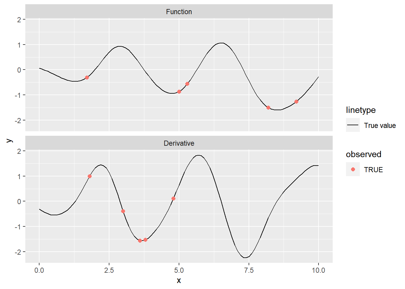

With the data combined into one long vector, the joint distribution of the observed data \(\bm{y}^{all}\) is now given by \[ \bm{y}^{all} \sim MVN\left(\bm{0}, k^{all}(\bm{x}^{all}, \bm{x}^{all}, \bm{d}^{all}, \bm{d}^{all}) \right) \]

where \(k^{all}\) is a function which computes the covariance between points, choosing the right covariance formula to use depending on if a point is a derivative or function value: \[ k^{\mathrm{all}}(x_i, x_j, d_i, d_j) = \begin{cases} k(x_i, x_j) & d_i = 0, d_j = 0 \text{ (both normal observations)} \\ k_{01}(x_i, x_j) & d_i = 0, d_j = 0 \text{ (one derivative, one normal)} \\ k_{10}(x_i, x_j) & d_i = 1, d_j = 0 \text{ (one derivative, one normal)} \\ k_{11}(x_i, x_j) & d_i = 1, d_j = 0 \text{ (both derivatives)} \end{cases} \]

We want to predict both the function values and derivatives at a set of new points \(\tilde{\bm{x}}\). Define \(\tilde{\bm{x}}^{all}\) to be a vector formed by repeating \(\tilde{\bm{x}}\) twice, with \(\tilde{\bm{d}}^{all} = \left\{0, 0, \cdots, 0, 1, 1, \cdots, 1\right\}\) indicating whether each element of \(\tilde{\bm{x}}\) refers to a function or derivative prediction.

x_tilde <- seq(0, 10, 0.1) # Prediction points

x_tilde_all <- c(x_tilde, x_tilde)
d_tilde_all <- c(rep(0, length(x_tilde)), rep(1, length(x_tilde)))

Fortunately, the conditional distribution of a multivariate normal distribution has a closed form. Applying the formula, we arrive at \[ \tilde{\bm{y}} \mid \tilde{\bm{x}}^{all}, \bm{y}^{all}, \bm{x}^{all} \sim MVN(\bm{K}^\top \bm{\Sigma}^{-1} \bm{y}^{all}, \bm{\Omega} - \bm{K}^\top \bm{\Sigma}^{-1} \bm{K}) \] where

• \(\bm{\Sigma}\) is the covariance matrix between observed points \(\bm{x}^{all}\)
• \(\bm{\Omega}\) is the covariance matrix between the new points \(\bm{\tilde{x}}\)
• \(\bm{K}\) is the covariance matrix between the observed points \(\bm{x}^{all}\) and new points \(\bm{\tilde{x}}\)

First, let’s compute each one of these matrices:

# Covariance between the observed points
Sigma <- joint_covariance_from_kernel(x_all, d_all, k_all, alpha = alpha, l = l)

# Due to computational floating point issues, it is sometimes necessary to
# add a small constant to the diagonal of Sigma to make sure it's not singular
Sigma <- Sigma + diag(1e-4, nrow(Sigma))

# Covariance between the prediction points
Omega <- joint_covariance_from_kernel(x_tilde_all, d_tilde_all, k_all, 
                                      alpha = alpha, l = l)

# Covariance between the observed and prediction points
# We calculate K by computing the covariance between x_all and x_tilde_all
K <- outer(
  1:length(x_all),
  1:length(x_tilde_all),
  function(i, j) {
    k_all(x_all[i], x_tilde_all[j], d_all[i], d_tilde_all[j], alpha = alpha, l = l)
  }
)

Then apply the conditioning formula to get the conditional mean and covariance matrix:

mu_conditional <- t(K) %*% solve(Sigma) %*% y_all
Sigma_conditional <- Omega - t(K) %*% solve(Sigma) %*% K

For plotting, it’s helpful to extract the marginal variances of each prediction, which are the diagonal entries of the conditional covariance matrix. We can also use this to get a 95% prediction interval:

variance_conditional <- diag(Sigma_conditional)

# Floating point errors sometimes causes the variances to be very close to zero, 
# but negative. If this happens, just set the variance to zero:
variance_conditional <- ifelse(variance_conditional < 0, 0, variance_conditional)

# 95% intervals
lower_bound <- mu_conditional - 1.96 * sqrt(variance_conditional)
upper_bound <- mu_conditional + 1.96 * sqrt(variance_conditional)

Let’s plot the result:

f_conditional <- tibble(
  x = x_tilde_all,
  d = d_tilde_all,
  y = mu_conditional,
  lower = lower_bound,
  upper = upper_bound
) 

ggplot(f_conditional, aes(x = x, y = y)) +
  geom_ribbon(aes(ymin = lower, ymax = upper), alpha = 0.2) +
  geom_line(aes(lty = "Conditional mean")) +
  geom_line(aes(lty = "True value"), data = f) +
  geom_point(aes(color = observed), data = filter(f, observed)) +
  scale_linetype_manual(values = c(2, 1)) +
  facet_wrap(~d, ncol = 1, labeller = labeller)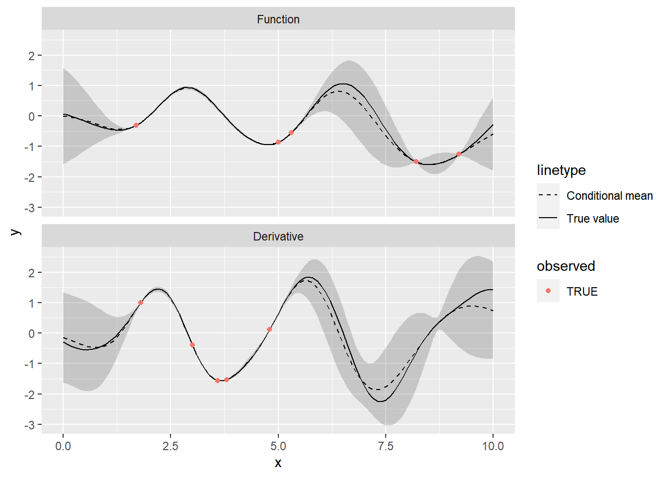

The inclusion of derivative information between \(x=2.5\) and \(x=5.0\) appears to have a big effect on the predictions. Even though there are no function values in this region, the derivatives are able to guide the predictions.

It would be nice to be able to compare these predictions to ones that don’t use any derivative information. To make this easier, let’s wrap up our code into a helper function which will handle the conditional multivariate normal calculations:

# To make this more readable I'm omitting the "_all" suffixes on variable names
condition_joint_gp <- function(x_tilde, d_tilde, y, x, d, kernel, ...) {
  Sigma <- joint_covariance_from_kernel(x, d, kernel, ...) +
    diag(1e-4, length(x))
  
  Omega <- joint_covariance_from_kernel(x_tilde, d_tilde, kernel, ...)
  
  K <- outer(1:length(x), 1:length(x_tilde),
          function(i, j) kernel(x[i], x_tilde[j], d[i], d_tilde[j], ...))
  
  mu_conditional <- (t(K) %*% solve(Sigma) %*% y)[, 1]
  Sigma_conditional <- Omega - t(K) %*% solve(Sigma) %*% K
  
  var_conditional <- diag(Sigma_conditional)
  var_conditional <- ifelse(var_conditional < 0, 0, var_conditional)
  
  tibble(
    x     = x_tilde,
    d     = d_tilde,
    y     = mu_conditional,
    var   = var_conditional,
    lower = y - 1.96 * sqrt(var_conditional),
    upper = y + 1.96 * sqrt(var_conditional)
  )
}

And let’s also wrap up the plotting code into a function:

plot_conditional <- function(f_conditional, f) {
  ggplot(f_conditional, aes(x = x, y = y)) +
    geom_ribbon(aes(ymin = lower, ymax = upper), alpha = 0.2) +
    geom_line(aes(lty = "Conditional mean")) +
    geom_line(aes(lty = "True value"), data = f) +
    geom_point(aes(color = observed), data = filter(f, observed)) +
    scale_linetype_manual(values = c(2, 1)) +
    facet_wrap(~d, ncol = 1, labeller = labeller)
}

Now let’s condition on just the function observations, leaving out the derivative points, and plotting the results.

non_derivative_indices <- which(d_all == 0)

f_conditional_no_derivatives <- condition_joint_gp(
  x_tilde_all,                   # Prediction points
  d_tilde_all,                   # Derivative indicator at prediction points
  y_all[non_derivative_indices], # Observed function values
  x_all[non_derivative_indices], # Position of observed values
  d_all[non_derivative_indices], # Derivative indicator of observed values
  k_all,
  alpha = alpha,
  l = l
)


# First, plot the predictions that don't use derivative information
plot_conditional(
  f_conditional_no_derivatives,
  mutate(f, observed = ifelse(d == 1, FALSE, observed))
) +
  ggtitle("Predictions without derivative observations")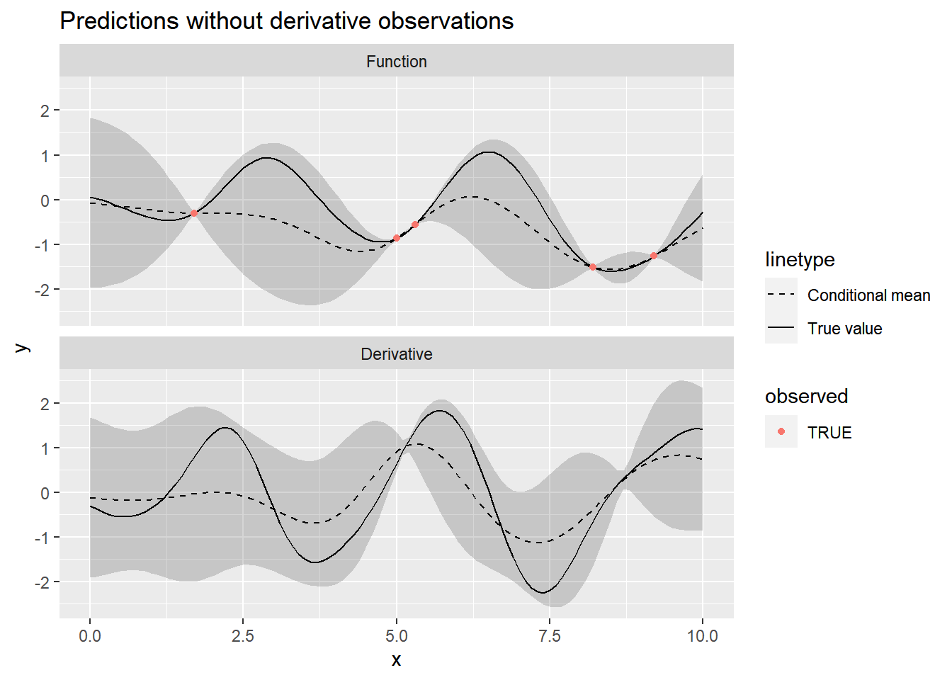

# Then plot again the predictions that use the derivatives
plot_conditional(f_conditional, f) +
  ggtitle("Predictions using derivative observations")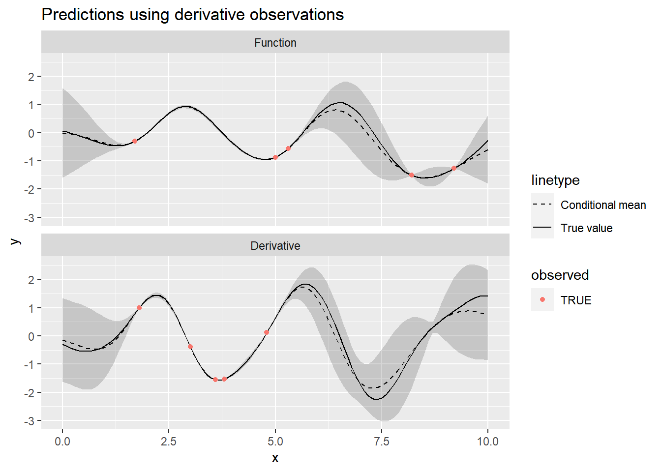

As we would expect, including more information by providing some derivative observations leads to much better predictions.

Up until now, we have been fixing the hyperparmaters of the Gaussian Process to known values. However, in the real world it’s rare to know these parameters; we need to estimate them. In a future post I’ll show how to use Stan to estimate the hyperparameter values using full Bayesian inference.