Derivative Gaussian Processes in Stan

Model Specification

Suppose we observe the vector \(\bm{y}^{all}\) at positions \(\bm{x}^{all}\), with \(\bm{d}^{all}\) indicating whether each element of \(\bm{y}^{all}\) is a function or derivative observation.

We will assume that \(\bm{y}^{all}\) are noisy measurements of the underlying function and its derivative. That is, \(y_i\) is normally distributed around the truth with a fixed error \(s^2\): \[ \begin{aligned} y^{all}_i &\sim \mathrm{N}(\mu_i, s^2) \\ \mu_i &= \begin{cases} f(x^{all}_i) & d_i = 0, \\ f^\prime(x^{all}_i) & d_i = 1 \end{cases} \end{aligned} \] In practice we might want to estimate the sampling variance as a separate parameter; for this post we will assume tha \(s\) is known.

We place a mean-zero Gaussian Process prior on \(f\) with a squared exponential kernel function \(k\): \[ \begin{aligned} f &\sim \mathcal{GP}(0, k(x_i, x_j)) \\ f^\prime &\sim \mathcal{GP}(0, k_{11}(x_i, x_j)) \end{aligned} \]

The kernel function is written \[ k(x_i, x_j) = \alpha^2 \exp\left(- \frac{(x_i - x_j)^2}{2\ell^2} \right) \] where \(\alpha\) sets the variance and \(\ell\) is a length-scale parameter.

We will predict the values of the function at a grid of points \(\bm{x}^{pred}\). We want to predict the function and its derivative, so we need another \(\bm{d}^{pred}\) to indicate whether each grid point corresponds to a funtion or derivative prediction. The Gaussian Process model implies that \[ \begin{aligned} f^{d_i}(\bm{x}^{pred}) \sim MVN\left(\bm{0}, k_{all}\left(\bm{x}^{pred}, \bm{x}^{pred}, \bm{d}^{pred}, \bm{d}^{pred} \right) \right) \end{aligned} \] where I’m kind of abusing notation a little bit, with \(f^{d_i}\) being either the function \(f\) or its derivative \(f^\prime\) depending on the value of \(d_i\). The overall idea here is that the fact that we placed a Gaussian process prior on \(f\) implies that the joint distribution of it and its derivative is multivariate normally distributed according to a big covariance matrix defined by the function \(k_{all}\).

To complete the model specification we need set priors on the kernel parameters \(\alpha\) and \(\ell\). The prior choice, particularly for \(\ell\), can be tricky; for a more thorough look at why this is and how to set priors in a principled manner I recommend the case study Robust Gaussian Process Modeling by Michael Betancourt. For this post we will set informative Gamma priors assuming we know that the true parameter values are \(\alpha=1\), \(\ell = 1\): \[ \begin{aligned} \alpha &\sim \mathrm{Gamma}(5, 5) \\ \ell &\sim \mathrm{Gamma}(5, 5) \\ \end{aligned} \]

Writing the Model in Stan

Recall that the kernel \(k^{all}\) takes two observations and returns their covariance depending on whether each observation is a function or derivative observation: \[ k^{\mathrm{all}}(x_i, x_j, d_i, d_j) = \begin{cases} k(x_i, x_j) & d_i = 0, d_j = 0 \text{ (both normal observations)} \\ k_{01}(x_i, x_j) & d_i = 0, d_j = 0 \text{ (one derivative, one normal)} \\ k_{10}(x_i, x_j) & d_i = 1, d_j = 0 \text{ (one derivative, one normal)} \\ k_{11}(x_i, x_j) & d_i = 1, d_j = 0 \text{ (both derivatives)} \end{cases} \] See the first post for the definitions of \(k\), \(k_{01}\), \(k_{10}\), and \(k_{11}\). In Stan we implement this as a function (in the functions block) which takes a vector x, with the argument derivative indicating whether each element of x corresponds to the function or its derivative.

To implement the Gaussian Process we use an efficient Cholesky Factored implementation. See the Gaussian Processes from the Stan User’s Guide for more details.

Also note a restriction of how this model is coded: we require that places the function is observed (\(x^{all}\)) is included in the grid of places where the function is predicted (\(\bm{x}^{pred}\)). This is so we can write the model to predict at all the points in \(\bm{x}^{pred}\) and then link those predictions to the observed data via the likelihood.

Here is the full Stan model:

functions {
  matrix kernel(real[] x, int[] derivative, real alpha, real rho) {
    int N = size(x);
    matrix[N, N] K;
    real sq_alpha = square(alpha);
    real sq_rho = square(rho);
    real rho4 = pow(rho, 4);
    
    real r = -inv(2 * sq_rho);
    
    for(i in 1:(N - 1)) {
      if(derivative[i] == 0) {
        K[i, i] = sq_alpha;
      }
      else if(derivative[i] == 1) {
        K[i, i] = sq_alpha / sq_rho;
      }
      
      for(j in (i + 1):N) {
        if(derivative[i] == 0 && derivative[j] == 0) {
          K[i, j] = sq_alpha * exp(r * square(x[i] - x[j]));
        }
        else if(derivative[i] == 0 && derivative[j] == 1) {
          K[i, j] = exp(r * square(x[i] - x[j])) * 
            (x[i] - x[j]) * sq_alpha / sq_rho;
        }
        else if(derivative[i] == 1 && derivative[j] == 0) {
          K[i, j] = exp(r * square(x[i] - x[j])) * 
            (x[j] - x[i]) * sq_alpha / sq_rho;
        }
        else if(derivative[i] == 1 && derivative[j] == 1) {
          K[i, j] = exp(r * square(x[i] - x[j])) * 
            (sq_rho - square(x[i] - x[j])) * sq_alpha / rho4;
        }
        K[j, i] = K[i, j];
      }
    }
    if(derivative[N] == 0) {
      K[N, N] = sq_alpha;
    }
    else if(derivative[N] == 1) {
      K[N, N] = sq_rho * sq_alpha / rho4;
    }
    
    return K;
  }
}
data {
  // Number of grid points
  int T; 
  
  // Grid point locations
  real pred_xs[T]; 
  
  // Indicator of whether each grid point refers
  // to a function or derivative value
  int<lower=0, upper=1> pred_derivatives[T];
  
  // Number of observations
  int<lower=1> N;
  
  // Observed outcomes
  vector[N] y; 
  
  // Index of observations in grid
  int<lower=1,upper=T> index[N]; 
  
  // Sampling variance
  real<lower=0> s;
}

transformed data {
  real delta = 1e-9;
  
  // Square of sampling variance
  real sq_s = square(s);
}

parameters {
  // Length scale parameter
  real<lower=0> rho;
  
  // Variance parameter
  real<lower=0> alpha;
  
  vector[T] eta;
}

transformed parameters {
  // Function predicted at grid points
  vector[T] f;
  
  {
    // Compute covariance kernel
    matrix[T, T] L_K;
    matrix[T, T] K = kernel(pred_xs, pred_derivatives, alpha, rho);

    // add small value to diagonal
    // for numerical stability
    for (t in 1:T)
      K[t, t] = K[t, t] + delta;

    L_K = cholesky_decompose(K);
    f = L_K * eta;
  }
}
model {
  // Priors
  rho ~ gamma(5, 5);
  alpha ~ gamma(5, 5);
  
  eta ~ std_normal();
  
  // Likelihood
  // The observations y should be normally
  // distributed around the function predictions.
  // The variable index tells us which values in f
  // correspond to the observations y.
  y ~ normal(f[index], s);
}

When I use Stan models in R I like to wrap up the code that calls Stan into a separate function so it’s easier to reuse multiple times.

#'
#' Fit a Gaussian Process with derivatives in Stan
#' 
#' @param stan_model RStan model object
#' @param x x-coordinates of the observed values
#' @param y observed values of the function or its derivative
#' @param derivative vector indicating if each value of y is a
#'                   function observation (0) or derivative (1)
#' @param pred_xs where to predict the function and its derivative
#' @param sampling_variance fixed sampling variance
#' @param ... additional arguments passed to Stan sampler
stan_gaussian_process_derivative <- function(
  stan_model, 
  x, 
  y,
  derivative,
  pred_xs,
  sampling_variance, 
  ...
) {
  
  if(length(x) != length(y) || length(y) != length(derivative)) {
    stop("x, y, and derivative arguments must have same length")
  }
  
  if(any(x %in% pred_xs == FALSE)) {
    stop("all values of x must be in pred_xs")
  }
  
  # Repeat the grid twice, first for function values
  # and second for its derivative
  grid <- c(pred_xs, pred_xs)
  derivative_grid <- c(rep(0, length(pred_xs)), rep(1, length(pred_xs)))
  
  # Map the observed xs to their positions in the prediction grid
  x_indices <- match(x, pred_xs)
  
  # the derivatives are in the second half
  # of the grid, so offset their positions
  x_indices <- ifelse(derivative == 1, x_indices + length(pred_xs), x_indices)
  
  # Make sure we did this step correctly:
  stopifnot(all(grid[x_indices] == x))
  stopifnot(all(derivative_grid[x_indices] == derivative))
  
  stan_data <- list(
    T = length(grid),
    pred_xs = grid,
    pred_derivatives = derivative_grid,
    N = length(x),
    y = y,
    index = x_indices,
    s = sqrt(sampling_variance)
  )
  
  fit <- rstan::sampling(stan_model, stan_data, ...)
  
  # Return the stan data object and the fitted model object
  list(
    data = stan_data,
    fit = fit
  )
}

It’s also convenient to write functions for summarizing the posterior distribution of the function predictions and for plotting the results.

To summarize the posterior, we use tidybayes to extract posterior medians and 95% credible intervals.

#' Summarize posterior medians and credible intervals of 
#' Gaussian Process derivative fit
#'
#' @param fit output from stan_gaussian_process_derivative function
summarize_gp_posterior <- function(fit) {
  tidybayes::spread_draws(fit$fit, f[index]) %>%
    mutate(x = fit$data$pred_xs[index],
           d = fit$data$pred_derivatives[index]) %>%
    group_by(d, x) %>%
    tidybayes::median_qi(f)
}

For plotting, we’ll take the summarized posterior and plot it along with the true function values and the observed data.

#' Plot the posterior distribution from the model fit
#' and compare to the true function and observed data
#' 
#' @param posterior output from summarize_gp_posterior function
#' @param f data frame containing true function values and observed data
plot_posterior <- function(posterior, f) {
  # Facet labeller
  labeller <- as_labeller(c("0" = "Function", "1" = "Derivative"))
  
  f_observed <- filter(f, observed)
  
  ggplot(posterior, aes(x = x)) +
    # Posterior distribution
    geom_ribbon(aes(y = f, ymin = .lower, ymax = .upper), alpha = 0.2) +
    geom_line(aes(y = f, linetype = "Posterior median")) +
    
    # True function
    geom_line(data = f, aes(x, y_true, linetype = "True function")) +
    
    # Observed data
    geom_errorbar(data = f_observed, 
                  aes(ymin = y_lower, ymax = y_upper), width = 0.1) +
    geom_point(data = f_observed, 
               aes(x, y, color = observed), size = 2) +
    
    scale_linetype_manual(values = c(2, 1)) +
    
    facet_wrap(~d, ncol = 1, labeller = labeller)
}

Example: Fitting Simulated Data

Let’s draw some simulated data from a Gaussian Process. We’ll use the same code as the previous post, with a slight change to make the observed data have normally distributed error.

set.seed(9)

# Set hyperparameters
alpha <- 1
l <- 1

# Points at which to observe the function and its derivative
x <- rep(seq(0, 10, 0.25), 2)
d <- c(rep(0, length(x) / 2), rep(1, length(x) / 2))

# Joint covariance matrix
Sigma <- joint_covariance_from_kernel(x, d, k_all, alpha = alpha, l = l)

# Draw from joint GP
y_true <- gp_draw(1, x, Sigma)[1, ]

# Add random error
sampling_variance <- 0.025
y <- rnorm(length(y_true), mean = y_true, sd = sqrt(sampling_variance))

Now let’s choose a few function and derivative values which we’ll use as our observed data:

# Pick a few function and derivative values to use as observed data, making
# sure to pick an equal number of each type
N <- 10
observed_indices <- c(
  sample(which(d == 0), N / 2),
  sample(which(d == 1), N / 2)
)

# We'll call the observed data y_all so that it matches with the math notation
x_all <- x[observed_indices]
y_all <- y[observed_indices]
d_all <- d[observed_indices]

Let’s plot the observed values with error bars, along with the true value of the function:

# Create a data frame for plotting
f <- tibble(
  x = x,
  y_true = y_true,
  y = y,
  y_lower = y - 1.96 * sqrt(sampling_variance),
  y_upper = y + 1.96 * sqrt(sampling_variance),
  observed = seq_along(x) %in% observed_indices,
  d = d
)

f_observed <- filter(f, observed)

labeller <- as_labeller(c("0" = "Function", "1" = "Derivative"))

ggplot(f, aes(x = x, y = y_true)) +
  geom_line(aes(lty = "True value")) +
  geom_errorbar(data = f_observed, 
                aes(ymin = y_lower, ymax = y_upper), width = 0.1) +
  geom_point(data = f_observed,
             aes(y = y, color = observed), size = 2) +
  facet_wrap(~d, ncol = 1, labeller = labeller) +
  ggtitle("True function and observed values")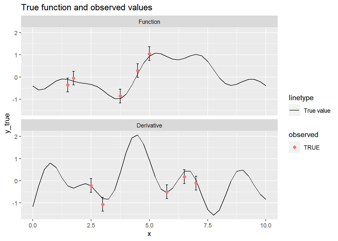

We can use the function we wrote to fit the model in Stan. We’ll run the sampling algorithm for 2,000 iterations, half of which are for warm-up.

stanfit <- stan_gaussian_process_derivative(
  model,
  x = x[observed_indices],
  y = y[observed_indices],
  derivative = d[observed_indices],
  pred_xs = x,
  sampling_variance = sampling_variance,
  
  # Sampling algorithm parameters
  iter = 2000,
  cores = 4
)

plot_posterior(summarize_gp_posterior(stanfit), f) +
  ggtitle("Gaussian Process Posterior")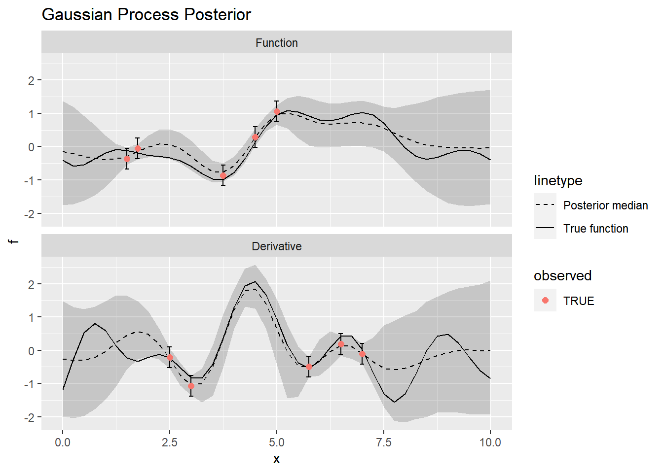

Let’s also check the posterior distributions for the kernel hyperparameters:

fit_matrix <- as.matrix(stanfit$fit)[, c("alpha", "rho")]

bayesplot::mcmc_recover_hist(fit_matrix, c(1, 1))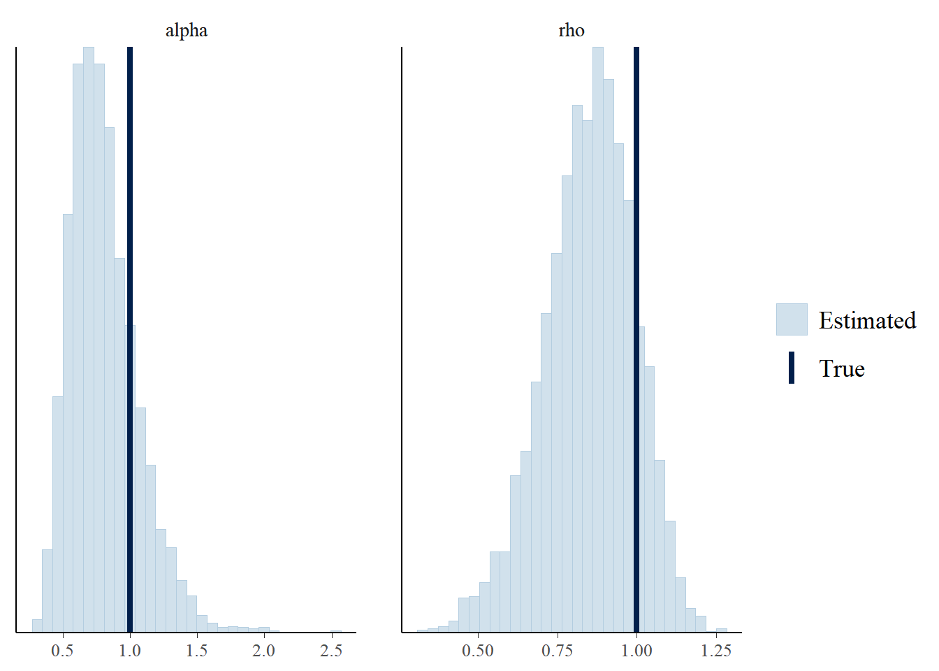

bayesplot::mcmc_recover_intervals(fit_matrix, c(1, 1))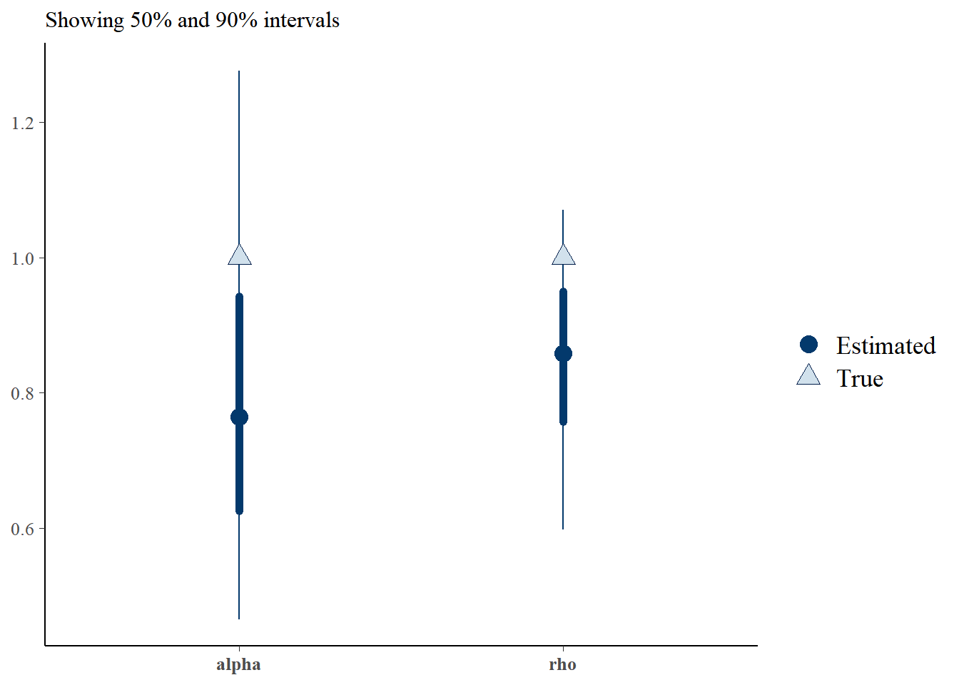

The posterior mode underestimates the hyperparameters, although the true values are well within the 90% credible intervals.

Let’s fit the model again, but this time leave out the derivative observations so we can see how much they influence the model fit. This is where wrapping up all the code into functions pays off, as we won’t need to rewrite all of the model fitting code.

observed_no_derivatives <- observed_indices[d[observed_indices] == 0]

stanfit_no_derivatives <- stan_gaussian_process_derivative(
  model,
  x = x[observed_no_derivatives],
  y = y[observed_no_derivatives],
  derivative = d[observed_no_derivatives],
  pred_xs = x,
  sampling_variance = sampling_variance,
  
  # Sampling algorithm parameters
  iter = 2000,
  cores = 4
)

Now we can compare the two model fits, with and without the derivative values observed.

plot_posterior(summarize_gp_posterior(stanfit), f) +
  ggtitle("With derivatives observed")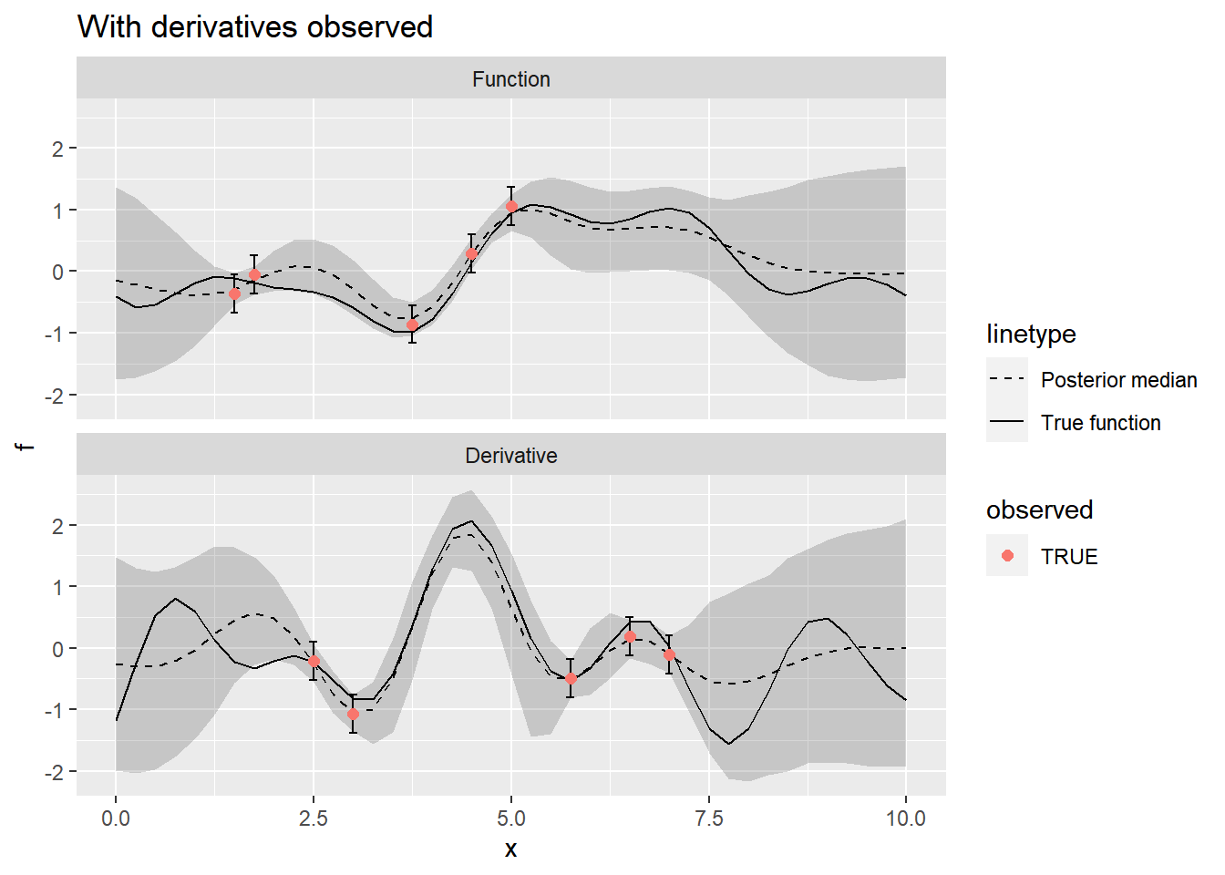

plot_posterior(
  summarize_gp_posterior(stanfit_no_derivatives),
  mutate(f, observed = ifelse(d == 0, observed, FALSE))
) +
  ggtitle("Without derivatives observed")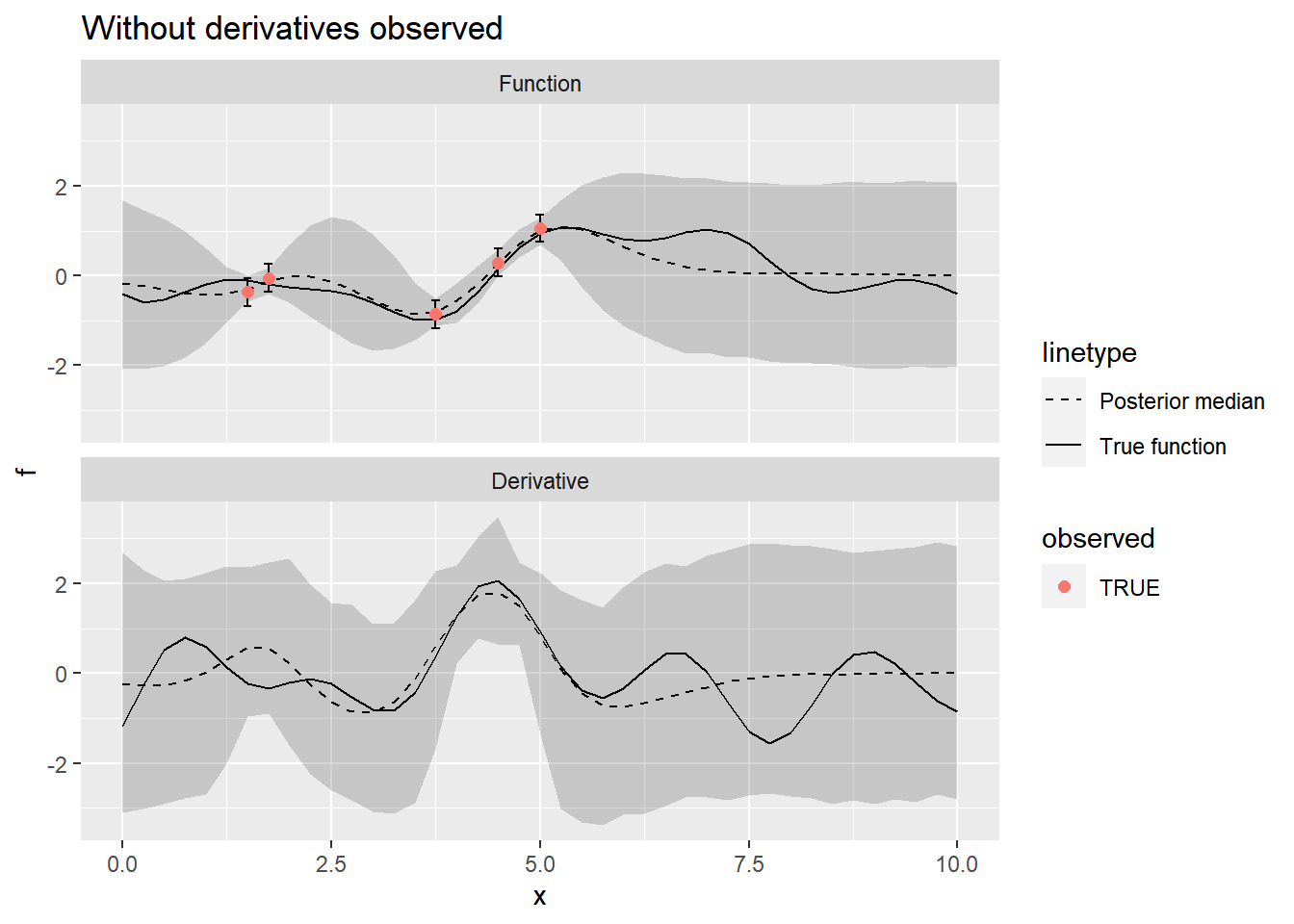

Including the derivative observations makes a big difference in the model fit, as we would expect.